Plastic forming processes of transverse non-homogeneous composite metallic sheets

1 Introduction

High importance exists for thin walled structures like sheets that play a pivotal role in the advanced modern industries. In the technological world the rising challenges for products, cause the various components of those products to fulfill simultaneous requirements. For instance, low weight on one hand and resistance to corrosion, fatigue and high thermal conductivity on the other hand. Most of the material in their raw form (we shall call them “homogenous”), satisfy one or two demands of the designer specifications, and thus the need for non-homogeneous materials is conceived.

In cases where the need for: production in large quantities, accuracy of dimensions of the final product and several design complex specification demands, are necessary, plastic forming processes are the answer.

There are several kinds of plastic forming processes for sheets production, including: rolling extrusion and drawing. In this work we shall research the later two. Forming in extrusion and drawing is usually done using a wedge shaped die.

The method that is customary in multi-layered composite production is high speed forming (i.e. explosion). Two metals are coupled together one on top of the other and above them an explosive layer. The shock wave that is created from the explosive's detonation, proceeds and creates a welding effect in the intermediate surface between the layers (see Figure 1). Other methods for creating multilayered materials are the plastic forming processes themselves (meaning not just forming the material but also manufacturing it).

Figure 1

Explosively welded multi-layered material (taken from [10]). (a) Cross section of a tri-layered sheet. (b) The shock wave of the explosion creates a wavy intermediate surface (taken from [8]). (c) A tri-layered sheet produced by using a cold plastic forming process of drawing and/or extrusion (taken from [6]).

It seems that in the practical reality described, there are several phenomena that occur to the homogenous material forming processes and belong also to the discussion of non-homogeneous materials. For example, in the extrusion process of homogeneous sheets the phenomenon of chevroning or central burst occurs. The raw material is inserted into a wedge shaped die and during the forming process, cracks are formed that assimilate in the final product. Therefore, although we are dealing with a homogenous material we have formed a non-homogeneous material. There are several other phenomena that we would like to understand, like: Bulging – where the material cannot advance in the die, dead zone formation and residual chips – cases where there is a branching of the flow pattern and a discontinuous shear surface is formed. In order to prevent these flaws from occurring it is necessary to generalize the method of the mathematical model solution's from one of homogenous material to a material with non-homogeneity.

When examining the works done in the domain of plastic forming processes the works [1, 11, 27] are recalled. The two-dimensional radial flow field that corresponds to sheet forming was first solved by Nadai [25] and Hill [18] for rigid/perfectly plastic material. Haddow & Danyluk [17] solved the flow field for an elastic/perfectly plastic material. Durban & Budianski [16] solved the flow field for rigid/plastic material with linear hardening, although this solution does not degenerate to the rigid/perfectly plastic model. In Durban [12, 13] this solution is generalized to a rigid/plastic with power law hardening material. This model is applied for various configurations for the simulation of the appropriate forming processes. There are also analytical solutions for the flow field for visco-plastic materials: Sandru & Camenschi [28] solved the flow field using stream function; DeVeries et al. [12] for special viscous material that includes the solution of Newtonian fluid and the rigid/perfectly plastic models as private cases; Durban [14] described the solution for visco-plastic model that assumes that the strain rate is composed from a plastic and viscous components. In Alexandrov et al. [3] the field was solved for general anisotropic material.

The analytical solutions for the radial flow that were mentioned in the chapter so far, were used in the literature for the simulation of the forming processes for: sheets and thin walled tubes with a static plug. Since there are difficulties in finding closed form analytical solutions, additional analytical approximated methods were developed such as the bounds methods of Prager & Hodge [26]. Related lower bound solution can be found in [15, 18, 25] and upper bound solution can be found in [29, 33]. Another method is using asymptotic expansions, Johnson [20] that rely on applied mathematics techniques and the use of perturbations.

Today in the industry there is an increasing trend of using multi-layered metallic materials. Broutman & Krock [8] reviewed the advantages using multi-layered materials. Blazynski & Dara [6] explain the process of multi-layered material that is implosively welded and in Broutman & Krock [8] the production is explained using rolling and extrusion. Blazynski & Townley [7] conducted experiments with bi-layered materials. Taheri [31] conducted experiments in tri-layered sheet drawing (not bonded) and compared to the solution in bounds methods. Szulc & Malinowski [30] solved for the same configurations using the finite elements method.

In plastic forming processes for radial two-dimensional flow pattern there are some phenomenon that do not agree with the analytical models. We shall mention bulging formation in sheets forming (Johnson & Rowe [21]), in certain configurations. This phenomenon was first reported by Hill [18, 19] that set the criterions for its appearance and showed that it happens where the velocity field derived (from the analytical solutions) is not physical (although the stress field is physical). Another phenomenon is residual chips and dead zones formation in extrusion of sheets that was studied by Tirosh [32]. In the range of large die angles there is bifurcation in the analytical flow field solution (Avitzur [4]). In these processes sometimes we encounter the phenomenon of chevroning (as was the case in Kudo [23]). Attempts to predict this phenomenon were made by Moritoki & Okuyama [24], Ko & Kim [22]. In general, it can be said that the appearance of flaws indicates the non-homogeneous influence of the material on the radial solution validity limit. It can be seen in Alexandrov et al. [2, 9] in the case of radial two-dimensional tri-layered symmetric sheet flow pattern, the influence of this phenomenon by finding configurations where there is no solution for the equations. There is also the examination of the loss of stability in the bonding zone between the layers in Bigoni et al. [5].

In this work, that is based on Davidi [10], we shall investigate the various forming processes in the case of continuous non-homogeneity of the material that will enable us to broaden the knowledge on these phenomena and find configurations to ensure their prevention.

2 Mathematical model

Lateral non-homogeneous sheet undergoes a plastic forming process of extrusion and drawing with large deformations through a wedge shaped die (see Figure 2) while reducing its thickness.

Figure 2

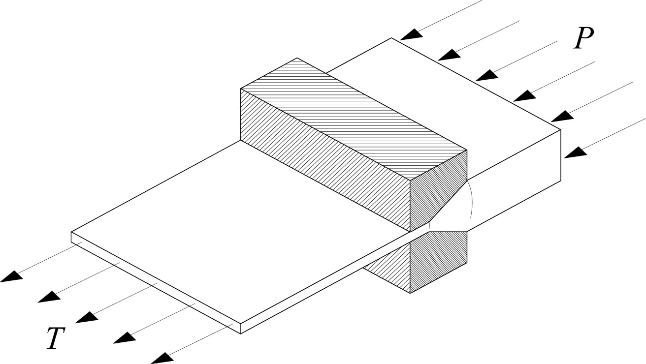
Forming process of a sheet through two wedge shaped dies.

The thickness of the sheet at the entrance to the dies is h_in and at the exit h_out (see Figure 3). The angles of the dies are α⁽¹⁾ and α⁽²⁾ respectively and the distance between the virtual apex “O” and the entrance is r_in and to the exit r_out. The reduction R is defined as the relative change in the cross section area between the entrance A_in and exit A_out and thus

In this work we shall deal with the specific symmetric case in which the angles are equal in size α⁽²⁾ = −α⁽¹⁾ = α.

Figure 3

Dimensions of the sheet and the wedge shaped dies in the process of drawing/extrusion.

The polar-cylindrical coordinate system (see Figure 4) will be used here where r and θ are the radial and meridian coordinates respectively and e_r and e_θ are the unit vectors. This coordinate system defines the walls of the dies by the surfaces θ = α⁽¹⁾ and θ = α⁽²⁾, together with surfaces r = r_in and r = r_out defines the working zone.

Figure 4

Polar-cylindrical coordinate system.

The set of equations according to continuum mechanics and plasticity associate to the flow theory (“J₂ flow theory”) include: equilibrium equations, the constitutive law of material and the kinematical relations. The equilibrium equations are

where σis the stress tensor. The constitutive law of a rigid/perfectly plastic material is

where S is the stress deviator tensor meaning,

p is the average stress, σ_e is the effective stress and D is the strain tensor. In this work we deal only with a rigid/perfectly plastic material and therefore we assume that

where Y is the yield stress of the material. It is convenient to use k, the yield stress in shear, instead of the yield stress Y, where it is known that

From equation (3) by double tensor multiplication it is possible to get the known expression to the effective stress

Now, we shall assume that k, the local yield stress in shear of the material, depends only on θ and the non-homogeneity is lateral, meaning, along the working zone thickness. Then, the kinematical relations are

where V is the velocity vector.

The boundary conditions are: A. Average working stress – the exact distribution of the extrusion and drawing stresses in the processes is unknown only their average values. Thus, the average extrusion stress employed at the entrance to the dies (see Figure 2) is

In the same way the drawing stress at the exit of the dies is

where Γ_T and Γ_P are the surfaces where the drawing and extrusion stresses are acting respectively, n is the unit vector normal to the surface and ds is the differential surface element.

We shall note here that the extrusion and drawing stresses are not independent and it is common to use the “loading parameter” η defined by

We shall mention that when η = 1 the process is pure drawing, when η = −1 the process is pure extrusion and when η > 1 the process is drawing with back pull - negative value of P in this case.

The next boundary condition is the friction at the walls dies – the “Siebel's friction” model, thus

where m is the friction coefficient and 0 ≤ m ≤ 1. k is the lowest value between the yield stress in shear of the surfaces in friction and the surface Γ_f is the surface in friction. According to definitions (12), τ_f cannot reach the value of the local yield stress in shear of the material.

The next boundary condition is the impermeable condition

where n_f is the unit vector normal to the surface Γ_f (see Figure 5).

Figure 5

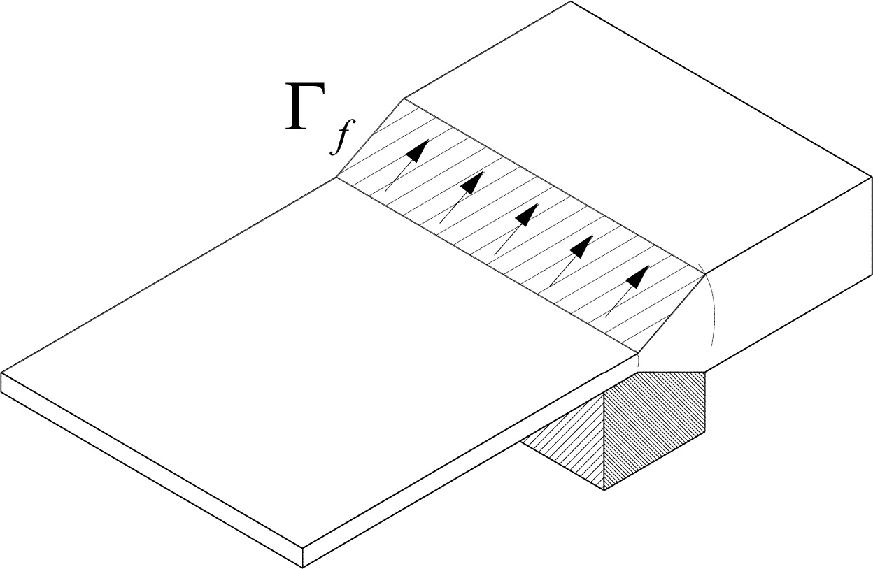
Boundary condition of friction with the walls of the dies. The upper wedge shaped die was removed to show the location of the friction.

The system of equations (2, 3, 4, 8) has no analytical closed form solution and in order not to solve the equations numerically (the whole set) we shall try to proceed with following set of assumptions:

A. Plane strain meaning

and then the stress σ_z in the case of rigid/perfectly plastic material is

B. Nadai-Hill assumption – this assumption states that the shear stress τ_rθ, does not change with the radial coordinate. We shall note that this assumption was used first by Nadai [25] and Hill [18] for the two-dimensional flow pattern and thus

Now, the rational behind this assumption (as described in Hill [25]) is that as long as we are far from the entrance and exit of the dies, the flow is approximately pure radial, and also τ_rθ along radial rays does not vary.

C. Negligence of inertial and body forces – it is assumed that the forming process is conducted in relatively quasi-static process (the material flow velocity is in the range of cm/sec). In this range of velocities it is fair to assume that we can omit dynamic and inertial terms.

D. Pure radial flow – we shall assume that the velocity vector V is of the form

We derived the system of equations (2, 3, 4, 8), boundary conditions (9, 10, 12, 13) and before approaching to find the solution we employ the set of assumptions on the mathematical model.

The equilibrium equations in cylindrical-polar coordinate system with the z component omitted due to the assumption of plane strain, are

The von-Mises yield criterion in this case is

and as we recall k is a function of only θ. We extract the expression σ_r − σ_θ from (19) and when selecting only the positive root, in our case σ_r > σ_θ, we get

we recall equilibrium equation (18) and apply Nadai-Hill assumption and get for equation (18) after dividing by 1/r, the form

We now integrate by θ and get

where g is an unknown function of r. We substitute the expression for σ_θ from equation (22) in equation (18) and get after integration by r

We substitute in equilibrium equation (18) equations (22) and (23) for σ_r and σ_θ and because the underlined terms are independent of r we get

Now, since in the equation (24) the underlined term depends solely on r and the double underlined term depends solely on θ

where C is constant and the derivative in equations (25, 26) is by θ. Now, we integrate equation (25) in order to derive the function g (r), we get

where D is an integration constant. Substituting (27) in expressions (22) to get σ_r and σ_θ respectively and we get

After solving equation (26) we can substitute τ_rθ in (28) that constitute explicit expressions for σ_r and σ_θ. We succeeded in finding the stress field without the need to find the velocity field first. This result is not surprising and actually there are infinite number of velocity fields that suit the stress field of solution of (26, 28). Because researching all field is not in the scope of this work we shall be satisfied with assumption D and thus have (17). The incompressibility condition that is derived from the kinematical relations in the von-Mises yield criterion, is

and after substituting the divergence operator in the cylindrical coordinate system with the velocity profile (17) we get that u is of the form

where f is an unknown function of θ and the negative sign suggests that the flow direction is towards the origin, the virtual apex “O”. In addition, the kinematical relations are

Now, the expressions for the deviator stresses S_r and S_rθ from (3, 4) can be calculated and from the parallel tensor property S//D, we get

and from (31) and (20) we thus get

and after integration by we get

and then u is known. Where Q is integration constant that represent the flow rate of the material.

We shall now turn to finding the working stress and the value of constant D. From (9, 10) the drawing and extrusion stresses are calculated

subtracting (36) from (35) we get

Now, substituting (28) for σ_r in (35, 36) we get the working stress T + P

Now, we find the constant D, by substitution of (35) and we get

We can express D by the loading parameter η from the loading parameter definition, expression (11), and have

The radial velocity is already known from (30, 34) where the constant Q calibrates the velocity vector component u, recalling that the problem is independent of time and thus Q is

where v_in and v_out are the velocities in the entrance and exit from the working zone.

To summarize, we now need to solve eq. (26) numerically (and calculate the constant C as mentioned previously), then calculate σ_r, σ_θ (28), σ_z (15), u (30, 34) using the expression for D from (40).

3 Case study

We now show interest in the process of a symmetric tri-layered sheet as a case study so we choose distribution of k (θ) accordingly. Let's suggest the follow distribution (shown in Figure 6). Due to symmetry it is sufficient to know the value of k for in half the region, meaning θ ∈ [0, α]. k₁ and k₂ are the values of k in the inner layer (core layer) and in the outer layer (cladding layer) respectively. This model enables for the first time to treat the intermediate surface and its influence on the solution. The location of the intermediate surface is θ = α₁. The thickness of the intermediate surface is α₂ (see Figure 6).

Figure 6

The distribution of a simple layered structure for k (θ): core, coating and an interface.

We shall assume that although the transition region between the two layers is not independent from r, it is fair to assume that an averaging can be made so that there is a region that depends only on (see Figure 7).

Figure 7

The intermediate interface between layers. Modeling the layer's interface as an average of material properties along lateral cross sections along the thickness of layer's interface (taken from [5]).

Now, we assume for the intermediate surface, meaning a sine like variation (the function sin is comfortable to work with, more than linear functions, because in addition to continuity of the function the derivative is also continuous for k (θ)). Therefore the distribution k (θ) is

We now turn to solving equation (26). The solution will be to numeric integrate τ_rθ by θ with the boundary conditions described earlier. We shall assume that the friction coefficient between the flowing material and the two wedge shaped dies are identical m₁ = m₂ = m and the boundary condition (12) is derived. Since the function is anti-symmetric with respect to θ = 0 then the boundary condition takes the form

Now, the integration of equation (26) is done by a shooting method (in order to set the constants C), using forth order Runge-Kutta scheme till the end of the domain, θ = α.

4 Results and discussion

The solution for equation (26) sometimes does not exist. This is due to the nature of it being an algebraic differential equation rather than a differential equation.

For the case of soft core and hard coating, α = 30°, α₁/α = 0.5, k₂/k₁ = 3.0 and α₂ = 0.1°, we can see the solutions in Figure 8 for different friction coefficients. It is shown that there is no solution for m > m_max = 0.33. Now, if we choose a ratio k₂/k₁ > 4.85 there is no solution to equation (26) for every possible boundary condition. In Figure 9 we map the ratio κ_SH = k₂/k₁|_max as a function of the process geometric configurations (α, α₁/α, α₂ = 0.1°).

Figure 8

Distribution of the normalized shear stress with the variation of θ and friction coefficient m, in the configuration: α = 30°, α₁/α= 0.5, α₂ = 0.1° and k₂/k₁ = 3.0.

Figure 9

The parametric envelope of the solution's validity limit, k_SH (α, α₁/α), in the case of tri-layered symmetric sheet.

In the same manner we show that for the case of hard core and soft coating for the configuration α = 30°, α₁/α = 0.5, k₁/k₂ = 5.5 and α₂ = 0.1° that there exists a solution for the range (see Figure 10). When plotting the value of κ_HS = k₁/k₂|_max as a function of α and α₁/α we see the result in Figure 11.

Figure 10

Distribution of the normalized shear stress, τ_rθ/k₂ with the variation of θ and friction coefficient m, in the configurations: α = 30°, α₁/α = 0.5, α₂ = 0.1° and for the ratio k₁/k₂ = 5.5.

Figure 11

The parametric envelope of the solution's validity limit, κ_HS (α, α₁/α), in the case of tri-layered symmetric sheet forming.

Another interesting result is the indifference of the validity limit of the solution in the intermediate surface thickness (expressed in α₂). This can be seen in Figure 12.

Figure 12

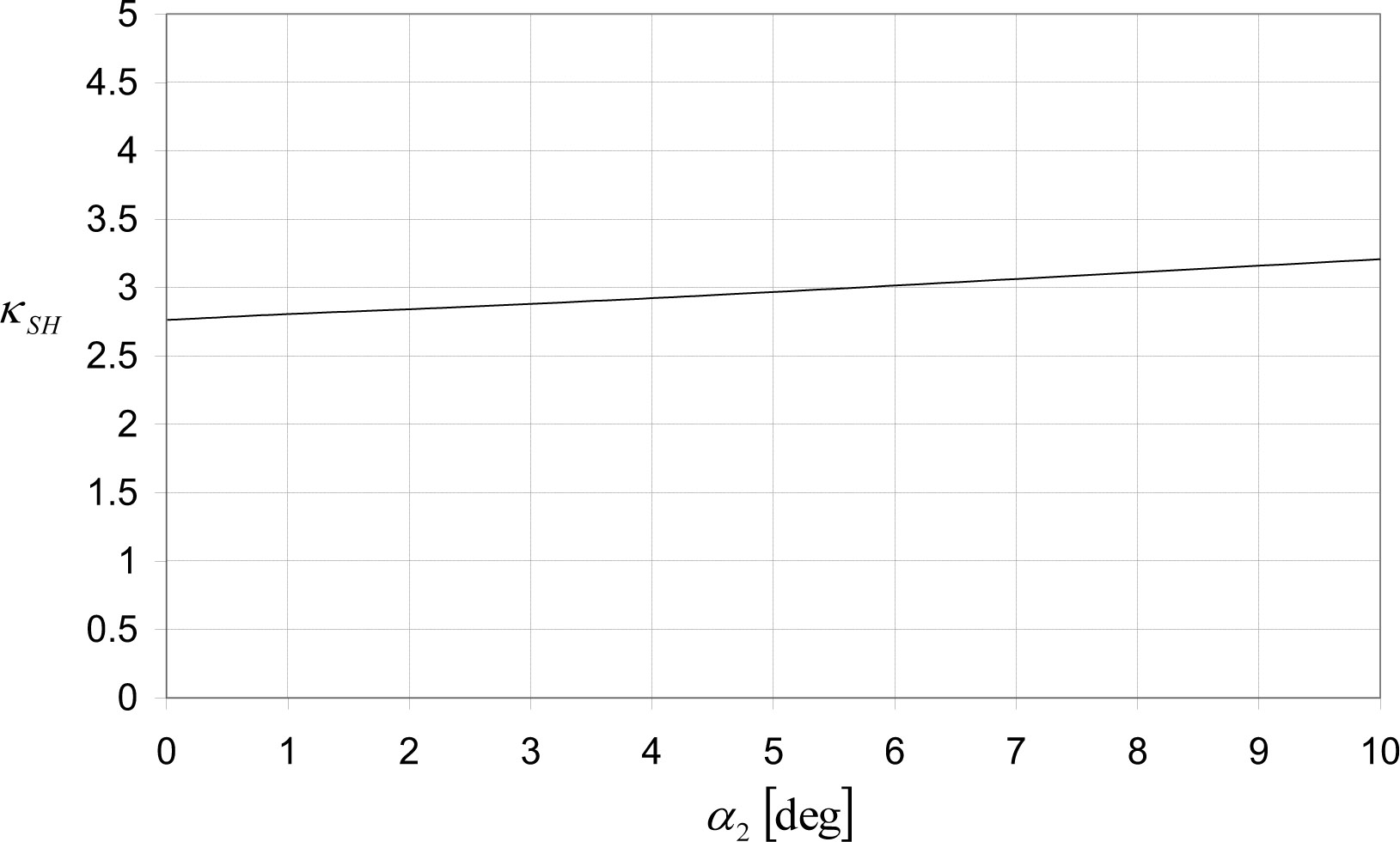
The effect of layer's interface thickness, α₂, on κ_SH, the validity limit of the radial solution. In this configuration: α = 60°, α₁/α = 0.5 in the process of tri-layered symmetric sheet forming.

It can be seen from Figures 9 and 11 that the validity limit of the radial solution is in the region of low die angle and in very thin cladding or very thin core. For high die angle or relatively thick cladding or thick core layers the solution is not radial and we should expect defects in the product of the forming process.

5 Summary and conclusions

From this research the following main conclusions:

1. The system of equations in their un-coupled form (equations 26, 28, 34) constitute a generalization of the known solutions of Nadai-Hill [18, 25] for a homogenous material, to a general transverse non-homogeneous material (across the working zone). Solution of this system degenerates to solution of a single non-linear first order algebraic differential equation (26) for the shear stress as a function of θ. The rest of the stress components and the radial velocity component are expressed explicitly as a function of the shear stress (equations 28).

2. From the examination of equation (26) it follows that the existence of solution is not always present for a given distribution k(θ)), across the working zone (this is due to the non-linear algebraic characteristic of the equation). In particular, in cases of a substantial difference in the yield stress of two adjacent layers it turns out that there is no solution to the equation. The results are that in simple layering (tri-layer symmetric sheet), the relative thickness of one layer to the other is also a parameter that affects the limit of the solution (see Figures 9, 11). When the intermediate surface location α₁/α is close to 0.5 the limit for the value of κ (the ratio of hardness of two adjacent layers) is the lowest. The effect of the angle α on the solution existence increase with increasing angle, meaning κ decreases with increasing α. In the case of small die angles κ ∞1 so there is no limitation on the solvability of the equations.

Figures 9 and 11 maps the “safe” configurations for which the radial solution holds thus the forming process will not produce defects as mentioned in the introduction.

References

[1] Alexander, J.M., and Brewer, R.C., “Manufacturing properties of materials,” Van Nostrand Reinhold company, 1963.Search in Google Scholar
[2] Alexandrov, S., and Mishuris, G., and Miszuris, W., “Planar Flow of a three – Layer Plastic Material Through a Converging Wedge-Shaped Channel, Part 1 – Analytical Solution,” European Journal of Mechanics and Solids, 2000, Vol. 19, pp. 811–825.10.1016/S0997-7538(00)01105-0Search in Google Scholar
[3] Alexandrov Sergei, Mustafa Yusof and Lyamina, Elena, “Steady planar ideal flow of anisotropic materials,” MECCANICA, 2016, vol 51, p. 2235–2241.10.1007/s11012-016-0362-xSearch in Google Scholar
[4] Avitzur, B., “metal forming: processes and analysis,” McGraw-Hill Book Company, 1968.Search in Google Scholar
[5] Bigoni, D., and Ortiz, M., and Needleman, A., “Effect of Interfacial Compliance on Bifurcation of a Layer Bonded to a Substrate,” International Journal of Solids and Structures, Vol. 34, 1997, pp. 4305–4326.10.1016/S0020-7683(97)00025-5Search in Google Scholar
[6] Blazynski, T.Z., and Dara, A.R., “The nature and types of Bonds in explosively - welded compund cylinders,” Metals and Materials, Vol. 6, pp. 258–262, 1972.Search in Google Scholar
[7] Blazynski, T.Z., and Townley, S., “The methods of analysis of the process of plug drawing of bimetallic tubing applied to implosively welded composites,” International journal of mechanical sciences, 1978, Vol. 20, pp. 785–797.10.1016/0020-7403(78)90100-5Search in Google Scholar
[8] Broutman, L.J., and Krock, R.H., “Composite Materials - Volume 4 Metallic Matrix Composites,” Academic Press, 1974.Search in Google Scholar
[9] Chung Kwansoo, Alexandrov Sergei, “Ideal flow in plasticity,” APPLIED MECHANICS REVIEWS, 2007, vol 60, p. 316–335.10.1115/1.2804331Search in Google Scholar
[10] Davidi, G., “Plastic forming processes of composite materials,” Scholars Press, 2013.Search in Google Scholar
[11] Degarmo, E.P., and Black, J.T., and Kohser, R.A., “materials and processes in manufacturing,” Prentice hall, 1988.Search in Google Scholar
[12] DeVries, G., and Craig, D.B., and Haddow, J.B., “Pseudoplatic converging flow,” International Journal of mechanical sciences, 1971, Vol. 13, pp.763–772.10.1016/0020-7403(71)90045-2Search in Google Scholar
[13] Durban, D., “on generalizes radial flow patterns of viscoplastic solids with some applications,” International Journal of mechanical sciences, 1986, Vol. 28, pp. 97–110.10.1016/0020-7403(86)90017-2Search in Google Scholar
[14] Durban, D., “On some simple steady forming process of viscoplastic solids,” Acta Mechanica, 1985, Vol. 57, pp. 123–141.10.1007/BF01176913Search in Google Scholar
[15] Durban, D., “Radial Flow Simulation of Drawing and Extrusion of Rigid/Hardening Materials,” International Journal of Mechanical Sciences, 1983, Vol. 25, pp. 27–39.10.1016/0020-7403(83)90084-XSearch in Google Scholar
[16] Durban, D., and Budiansky, B., “Plane-strain radial flow of plastic materials,” Journal of mechanical physics of solids, 1979, Vol. 26, pp. 303–324.10.1016/0022-5096(78)90002-9Search in Google Scholar
[17] Haddow, J.B., and Danyluk, H.T., “The Flow of an Incompressible Elastic-Perfectly Plastic Solid,” Acta Mechanica, 1968, Vol. 5, pp.14.10.1007/BF01624440Search in Google Scholar
[18] Hill, R., “The Mathematical Theory of Plasticy,” Oxford, 1950.Search in Google Scholar
[19] Hill, R., and Tupper, S. J., “A New Theory of the Plastic Deformation in Wire-Drawing,” Journal of the iron and steel institute, 1948, pp. 353–359.Search in Google Scholar
[20] Johnson, R.E., “Conical extrusion of a work-hardening materials: an asymptotic analysis,” Journal of engineering mathematics, 1987, Vol. 21, pp. 295–329.10.1007/BF00132681Search in Google Scholar
[21] Johnson, R.W., and Rowe, H.G., “Bulge Formation in Strip Drawing with Light Reductions in Area,” Proceedings of the Institution of Mechanical engineers, Vol. 182, 1967–1968, pp. 521–529.10.1243/PIME_PROC_1967_182_040_02Search in Google Scholar
[22] Ko, D. C. and Kim, B. M., “The Prediction of Central burst defects in Extrusion and Wire Drawing,” Journal of material processing technology, Vol. 102, 2000, pp. 19–24.10.1016/S0924-0136(99)00461-6Search in Google Scholar
[23] Kudo, H., “Some Analytical and Experimental Studies of Axisymmetric Cold Forging and Extrusion, Part I and II,” International Journal of Mechanical Sciences, 1960, Vol. 2, pp. 102–127, 1961, Vol. 3, pp. 91–117.10.1016/0020-7403(60)90016-3Search in Google Scholar
[24] Moritoki, H., and Okuyama, E., “Prediction of Central Bursting in Extrusion,” Journal of Materials Processing Technology, Vol. 80–81, 1998, pp. 579–584.10.1016/S0924-0136(98)00165-4Search in Google Scholar
[25] Nadai, A., “Uber die Glut- und Verzweigungsflachen einiger Gleichgewichtszustande bildsamer Massen und die Nachspannungen bleibend verzerrter Korper.,” Z. Phys., 1924, Vol 30, pp. 106–138.10.1007/BF01331828Search in Google Scholar
[26] Prager, W., and Hodge, P., “Perfectly plastic solids,” John Willey & sons Inc, 1951.Search in Google Scholar
[27] Radford, J.D., and Richardson, D.B., “Production engineering technology,” Macmillan press LTD, 1974.Search in Google Scholar
[28] Sandru, N., and Camenschi, G., “Viscoplastic Flow Through Inclined Planes with Application to the Strip Drawing,” Applied Engineering Sciences, 1979, Vol. 17, pp. 773–784.10.1016/0020-7225(79)90052-1Search in Google Scholar
[29] Stepanskii, L.G., “The Boundaries of the Area of Plastic Defomation in Extrusion,” Rssion Engineering Journal (English Translation), 1963’ issue 9, pp. 40–42.Search in Google Scholar
[30] Szulc, W., and Malinowski, Z., “Theoretical and Experimental Investigation of the Multilayer tube Drawing,” Journal of material processing technology, Vol. 45, 1994, pp. 347–352.10.1016/0924-0136(94)90364-6Search in Google Scholar
[31] Taheri A.K., “Analytical study of drawing of non-bonded trimetallic strips,” 1993, Vol. 33, pp. 71–88.10.1016/0890-6955(93)90065-3Search in Google Scholar
[32] Tirosh, J., “On the Dead-Zone Formation in Plastic Axially-Symmetric Converging Flow,” Journal of mechanics and physics of solids, Vol. 19, 1971, p. 39–47.10.1016/0022-5096(71)90034-2Search in Google Scholar
[33] Tirosh, J., and Iddan, D., “The dynamics of fast metal forming processes,” Journal of the physics of solids, 1994, Vol. 42, No. 4, pp. 611–628.10.1016/0022-5096(94)90054-XSearch in Google Scholar
© 2021 Gal Davidi, published by De Gruyter
This work is licensed under the Creative Commons Attribution 4.0 International License.