
Abstract
The steady increase in the number of road users and their growing mobility mean that the issue of road safety is still a topical one. Analyses of factors influencing the number of road traffic accidents contribute to the improvement of road safety. Because changes in traffic volume follow a daily rhythm, hour of the day is an important factor affecting the number of crashes. The present article identifies selected mathematical models which can be used to describe the number of road traffic accidents as a function of the time of their occurrence during the day. The study of the seasonality of the number of accidents in particular hours was assessed. The distributions of the number of accidents in each hour were compared using the Kruskal-Wallis and Kolmogorov-Smirnov tests. Multidimensional scaling was used to present the found similarities and differences. Similar hours were grouped into clusters, which were used in further analysis to construct the ARMAXmodel and the Holt-Winters model. Finally, the predictive capabilities of each model were assessed.
1 Introduction
According to the World Health Organization (WHO), around 1.35 million people die in road traffic accidents each year, costing most countries about 3% of their gross domestic product. Road injuries are the leading cause of death in children and young adults aged 5–29 years, with more than half of all fatalities being among pedestrians, cyclists, and motorcyclists [1].
The high mortality rate, and the high cost of road crashes, make road traffic safety an important problem, the various aspects of which are widely discussed in the literature. Researchers try to identify factors that affect the level of road safety,which vary depending on the area studied, a country’s road traffic history [2], and road infrastructure and superstructure, etc. Because risk factors differ from one region to the next, analyses should be conducted at a local level, as a basis for more general joint discussions.
The main factors that contribute to the large number of road accidents include traffic volume [3] and inappropriate driver behaviours such as overspeeding, rash driving, non-compliance with traffic rules, carelessness while crossing roads, playing on road, alcohol intake, fatigue, and sleepiness [4, 5]. The authors of [6] analysed the problem of crashes from the perspective of the driver’s age, noting that risk factors such as lack of experience and skills, and risky driving behaviours were associated with young drivers, while problems such as visual, cognitive and mobility impairments were mainly found in older drivers. In turn, the authors of [7] believe that the main causes of road traffic accidents are associated with the lack of control and inadequate enforcement of road traffic laws (especially speeding, drink-driving, failure to respect the rights of other road users – mainly pedestrians and cyclists – and unsafe road infrastructure. [8] accents the role of tourist attractiveness of a region as a factor that significantly increases the number of road accidents, while [9] mentions key risks such as vehicle overloading, speeding, and drink-driving.
In [10], the following factors affecting accidents were taken into account: the cause of the accident, the genders of the victims, the number and type of vehicles involved in the accident, the time of the accident, the severity of the accident, the type of accident and the age group of the driver(s). In [11], Khan et al. enumerate the following as the main causes of accidents: distractions, different weather conditions, sleep deprivation, unsafe lane changes, night-time driving. A different approach was proposed in [12], where the severity of accidents and not their numbers was adopted as the dependent variable. The results showed that it was affected by the season, age of the driver, time of day, as well as road type and quality.
In some publications, road accidents are analysed taking into account the clock time of the occurrence of the crash. For example, the authors of [13, 14] investigated the impact of the time of the day during which the accident occurred on the driver’s drowsiness and the likelihood of the driver falling asleep at the wheel. In [15], the authors calculated the absolute risk and the relative risk of dying in a road accident at specific times of the day. The daily pattern of road accidents, along with other risk factors leading to crashes, was also investigated in [16, 17, 18]. In [18] the authors performed a spatial-temporal analysis, assessing not only the time of the event, but also the day of the week and the season of the year in which the crashes took place.
Clock time analyses allow to determine the time of the day at which the risk of road traffic accidents is the greatest, making it possible to implement preventive programs focused on this critical time. In view of this, the goal of this present study was to assess the clock-time related risk of road traffic accidents in Poland.
The research hypothesis assumed that the clock hour had a significant impact on the number of accidents. The hypothesis was thus formulated on account of the great interest of various organizations, including non-governmental and social organizations, dealing not only with road safety, but primarily the impact of the time of day on the accident rate on Polish roads. This interest results from the traditional lifestyle of the inhabitants of Poland. Therefore, the research focused mainly on the analysis of the impact of the time of day on road safety in Poland. Therefore, the objective of the article was to analyse this one variable that has an impact on accidents in road traffic, even though the number of accidents is also affected by other factors. Another argument in favour of this approach was the fact that the time of day is a constant factor for the entire country (it does not change depending on the area, unlike road traffic). It reflects well the way society functions and its lifestyle. Moreover, knowledge about the time is generally available and thus allows easy interpretation of the obtained results as well as inference. The proposed method can easily be applied to other countries or smaller administrative areas (e.g. in provinces or cities).
Multivariate analyses yield good predictive results, however, they require complicated and complex models [4, 6, 12], whichmay hinder their correct interpretation and/or require specialized computational programs. Information on some variables influencing the level of road safety is not widely disseminated, and measurement results are difficult to obtain or parameters are not monitored. Therefore, the advantage of the study presented in the article is also the ease and possibility of adapting the presented method in other, similar analyses.
It should also be emphasized that most of the considerations presented in the literature concern the statistical analysis of the variables affecting road accidents. The statistical significance and strength of individual factors are examined, however, on the basis of the obtained results, no mathematical models enabling prediction are constructed, which has been done in the present article.
In the first stage of the study, the seasonality of the number of accidents at particular hours was assessed. The Kruskal-Wallis and Kolmogorov-Smirnov statistical tests were used to compare the distribution of the number of accidents in each hour. The similarities and differences found were presented using multidimensional scaling. On this basis, similar hours were grouped in clusters, which were used in further analysis to construct the ARMAX model and the Holt-Winters model. Finally, each of the proposed models was evaluated, their predictive abilities were compared, and final conclusions were formulated.
The presented study follows the literature trend that postulates the need to constantly review and update the results regarding the impact of individual factors on road hazard [6] and the WHO’s 2030 Agenda for Sustainable Development, which aims to halve the global number of road deaths and injuries by 2030 [1].
2 The problem of road traffic accidents in Poland
Located on the East-West transport route, Poland is a country with a lot of transit transport, which strongly affects the intensity of its road traffic. According to the data of the Polish Border Guard Headquarters, in 2018 (the year of the present study), 12 435 345 vehicles entered Poland through the EU’s external borders [19]. This undoubtedly affected the number of road traffic accidents, which was 31 674 in Poland in 2018. As a result of those crashes, 2 862 people died and 37 359 were injured (including 10 941 seriously injured). Compared to the previous year 2017, the number of road traffic accidents was smaller by 1 086 (−3.3%), which is a positive result that follows the downward trend observed in the recent years (Figure 1).

Number of accidents in Poland in 2010–2019
Unfortunately, the reduction in the number of road traffic accidents did not lead to a reduction in the number of fatalities, which has been increasing over the last few years (Figure 2)

Road traffic fatality rates for 2010–2019
The statistics cited above show that the problem of road safety in Poland is topical and requires continuous measures to reduce the number of accident victims, as well as the social and economic consequences of such events.
3 Seasonality study
Let {xt}1≤t≤8760 be a numerical sequence representing the number of accidents in the following hours of each day of 2018. We divide this sequence into 24 subsequences ck = x24(j−1)+k+11≤j≤365, each of which corresponds to the number of accidents for a specific hour of the day k (let us assume that k = 0,1, . . . , 23) [20] e.g. the subsequence c0 contains data on the number of accidents that took place at zero hour (i.e. between 00:00 and 00:59) in the successive days of 2018. Figure 3 shows box-and-whisker plots for each group corresponding to a clock hour, while Figure 4 shows a chart of the seasonality of accidents as a function of time.

Box-and-whisker plot for road traffic accidents recorded in 2018
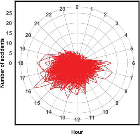
Chart showing the number of road traffic accidents in 2018
The above figures clearly show that the sequence exhibits seasonal changes, which are analysed statistically below.
4 Kruskal–Wallis test
The Kruskal–Wallis test was performed to test seasonality (the test was used to compare between groups) [21]. Let {ck}0≤k≤23 be a set of sequences corresponding to the number of accidents for a given hour of the day k. To examine seasonality at the level of significance α ∈ (0, 1), we formulated the following working hypothesis:
H0: the distributions of the number of accidents are the same for each hour of the day (i.e. the time of day does not affect the number of accidents),
and an alternative hypothesis:
H1: there are hours during the day for which the distributions of the number of accidents differ significantly.
Let n = n0 + n1 + . . . +n23 denote sample size (i.e. the number of elements in set {ck}0≤k≤23), which is divided into 24 disjoint groups of size n0 = n1 = ·· · = n23 (group sizes correspond to the respective hours of the day). Each group is randomly selected from a different population. The entire sample (all groups together) is ranked. Let Rij denote the rank in a sample of the j-th element from the i-th group.
The test statistic is given by the formula:
where:
Test statistic T (1) is a measure of deviation of rank mean of samples (groups) from the mean value of all ranks is equal (n+1)/2. Statistic T has distribution χ2 with 23 degrees of freedom.
The value of the test statistic is estimated at 4630.58, and p-value is < 2.2 · 10−16. This means that the distributions of the number of accidents differ significantly for different hours of the day.
5 Kolmogorov-Smirnov test
The Kolmogorov-Smirnov test was also used to compare the distributions of the number of accidents for each hour of the day [21, 22]. At significance level α ∈ (0, 1), the following working hypothesis was formulated for hours i and j (0 ≤ i, j ≤ 23, i ≠j):
H0: the cumulative distribution functions for the number of accidents for hours i and j are identical,
The alternative hypothesis was:
H1: the cumulative distribution functions for the number of accidents for hours i and j are significantly different.
The test statistic is given by the formula:
where Fi(t) and Fj(t) denote cumulative distribution functions for hours i and j, respectively. Statistic Dij has a Kolmogorov distribution. The critical value Kα is determined from the Kolmogorov distribution tables for the significance level α. If
At the significance level α = 0.01, there are no grounds to reject the null hypothesis for the following pairs of hours: 00:00-01:00, 00:00-04:00, 01:0002:00, 01:00-03:00, 01:00-04:00, 02:00-03:00, 02:0004:00, 05:00-22:00, 06:00-21:00, 07:00-08:00, 07:0009:00, 08:00-09:00, 09:00-10:00, 10:00-11:00, 10:00-12:00, 10:00-19:00, 11:00-12:00, 11:00-13:00, 11:00-19:00, 12:00-13:00, 12:00-19:00, 13:00-14:00, 13:00-18:00, 14:00-15:00, 14:00 -16:00, 14:00-18:00, 15:00-16:00, 15:00-17:00, 15:00-18:00, 16:00-17:00; the working hypothesis should be rejected in favour of the alternative hypothesis for the remaining pairs of hours.
Figure 5 shows the values of the Kolmogorov-Smirnov test statistic for comparing distributions between groups.

Values of the Kolmogorov-Smirnov test statistic for pairs of hours
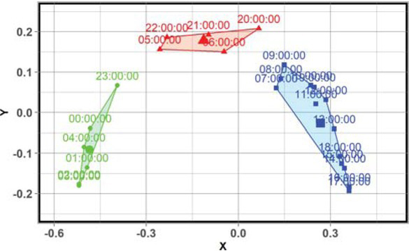
The values of the Kolmogorov-Smirnov test statistic on their own do not allow to group similar groups into clusters. To determine clusters, we used the Multidimensional Scaling Method followed by K-means Cluster Analysis.
6 Multidimensional Scaling
To present the similarities and differences of accident distributions between hours (objects) we employ the multidimensional scaling (MDS) [23, 24, 26]. It is a statistical technique, which allows us to visualize the similarities of individual groups. All differences between analysed groups are contained in a distance matrix. The Kolmogorov-Smirnov statistic (2) was used as the distance between distributions of accident. The multidimensional scaling tends to locate the objects as points in space, where the similar elements are located close together [23, 24].
The multidimensional scaling seeks the points zi ∈ R2, 1 ≤ i ≤ n that correspond to objects. By solution of the task:
we estimate the points corresponding to groups. Objective function:
is called a stress function, ║║ is an Euclidean norm.
Figure 6 presents the location of the groups estimated by applying multidimensional scaling method due to the Kolmogorov-Smirnov distance.
Cluster visualization
7 K-means cluster analysis
The K-means clustering method (see e.g. [24]) consists in partitioning an unlabelled data set into non-overlapping clusters and determining the centres of the clusters. Initially, we establish the number of clusters K. Let C = zj1≤j≤n denote a set of points corresponding to hours. zj ∈ R2. The task of the clustering method is to divide the entire C set into subsets called clusters C1, . . . , CK, where C1 ∪ . . . ∪ CK = C and Ci ∩ Cj = ∅ for i ≠j and 1 ≤ i, j ≤ K. For cluster Ck, 1 ≤ k ≤ K, we within-cluster variation is defined as follows
where ∥∥ is an Euclidean norm, |Ck| – number of objects in k−th cluster. The main idea of clustering consists in dividing the data set into clusters so that the sum of within-cluster variations (5) will be as small as possible. To determine the clusters we must solve the optimization task:
The result of K-means clustering application for locations obtained from the solution of the task (3) is as follows:
Cluster 1: 07:00, 08:00, 09:00, 10:00, 11:00, 12:00, 13:00, 14:00, 15:00, 16:00, 17:00, 18:00, 19:00;
Cluster 2: 00:00, 01:00, 02:00, 03:00, 04:00, 23:00;
Cluster 3: 05:00, 06:00, 20:00, 21:00, 22:00.
The location of the points (corresponding to hours) with clusters is presented in Figure 6. Each point is marked in XY coordinate systems, where X and Y denote the latent variables, which can be correlated with physical, weather-related and other factors.
8 ARMAX model
The number of road traffic accidents depends on the hour of the day, and hours are directly related to classes (clusters). To determine the dependence between number of accidents, hour of the day and other external factors which cannot be taken into consideration due to the lack of historical data, we consider the ARMAX (p, q) (AutoRegressive and Moving Average with external regressors) model. As a factor which directly influences on the number of incidents we take into account predictors describing membership in specific classes. The predictors are defined as binary variables that describe membership in classes 2 and 3, i.e.
and
We analyse a model given by:
where yt = log(xt + 1), 1 ≤ t ≤ 8760, B− backshift operator (for any k ∈ N, Bkyt = yt−k) and {ϵt}1≤t≤8760 is a sequence of independent random variables with a normal distribution N(0, σ2). We select from among the set of models (7), the one with the lowest AIC (Akaike Information Criterion) index. The model with lowest AIC is ARMAX(2.2). Table 1 presents the values of the estimators, standard deviations of the estimators, T statistics and probability for the working hypothesis that the value of estimator is equal to zero.
Estimator values and standard deviations of estimators.
| Estimator | Std. Error | T | p.value | |
|---|---|---|---|---|
| β1 | 1.6108 | 0.0481 | 33.4773 | < 2.2·10−16 |
| β2 | −0.6877 | 0.0397 | −17.3133 | < 2.2·10−16 |
| θ1 | −1.3666 | 0.0506 | −26.9898 | < 2.2·10−16 |
| θ2 | 0.5032 | 0.0338 | 14.8897 | < 2.2·10−16 |
| α0 | 0.5172 | 0.0188 | 27.5291 | < 2.2·10−16 |
| α1 | 1.1407 | 0.0245 | 46.5931 | < 2.2·10−16 |
| α2 | 0.6020 | 0.0184 | 32.7844 | < 2.2·10−16 |
Table 1 shows that at significance level 0.01 the working hypothesis should be rejected in favour of the alternative hypothesis. Thus, all estimator values are significantly different from zero. The value of the AIC index is 1325.406 and the value of the estimator σ2 is 0.266. Figure 7 shows empirical values of the transformation of the number of accidents (marked in black) and the values fitted with the model (7) (marked in red).

Empirical values and ARMAX(2.2) model fitted values
Figure 8 shows goodness of fit of residual distribution εt to normal distribution N(0, 0.266).

Goodness of fit of the residual distribution of the ARMAX(2,2) model to normal distribution
Additionally, the Kolmogorov-Smirnov residual normality test was performed. Value of the test statistics D is 0.035 and p-value is 7.46 · 10−10. This means that, at the significance level of 0.01, the working hypothesis should be rejected in favour of the alternative hypothesis.We also performed the Wald-Wolfowitz runs test [21]. Because the value of the Z statistic was −2.527, and p-value was 0.012, the working hypothesis regarding the randomness of the residuals should also be rejected at significance level 0.01.
The analysis of the distribution of residuals shows that it is not consistent with the normal distribution. Inclusion of additional predictors in the ARMAX model could improve the goodness of fit.
9 Holt-Winters method
The Holt-Winters method is a generalization of Brown’s exponential smoothing method [25, 27, 28, 29, 30]. It consists in estimating the trend and seasonality in a time series {xt}0≤t≤N. This method was proposed by Holt (estimation of trend [29]) and Winters (who extended it to the seasonality component [30]).
Consider time series {yt}1≤t≤8760 with additive seasonality of period p ∈ N given by
where
The values of estimators for level, slope and seasonality are determined from the formulas:
where 0 ≤ α, β, γ ≤ 1 stand for smoothing parameters.
The forecast (expected value) for 0 < k ≤ p moments ahead was determined based on the observation at moment t using the equation
Figure 9 shows empirical values of the transformation of the number of accidents log(xt + 1) (marked in black) and values fitted with the Holt-Winters model (marked in red).

Empirical values and Holt-Winters model fitted values
Values of smoothing parameters: α = 0.094, β = 0.005, γ = 0.07. The value of intercept estimator at = 1.169, the value of slope bt = −7.476·10−4. The estimator of variance of residuals ϵt in equation (8) is equal to 0.265. A seasonality curve for the Holt-Winters model is shown in Figure 10.
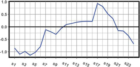
Seasonality curve for the Holt-Winters model
Figure 11 shows goodness of fit of the distribution of residuals ϵt. Additionally, the Kolmogorov-Smirnov residual normality test was performed. The value of the D statistics was 0.0213 and p-value was 7.034 · 10−4. This means that, at the significance level of 0.01, the working hypothesis should be rejected in favour of the alternative hypothesis. We also performed the Wald-Wolfowitz runs test. The value of the Z statistic was −8.385 and the p-value was < 2.2 · 10−16 and so the working hypothesis regarding the randomness of the residuals should also be rejected at significance level 0.01.

Goodness of fit of the residual distribution of the Holt-Winters model to the normal distribution
The Holt-Winters model which takes into account only the hour of the event also shows that there are other factors besides seasonality that directly affect the number of road traffic accidents, the inclusion of which could improve the quality of the model.
The constructed models are of similar quality (Table 1).
Goodness of fit of ARMAX and H-W models
| ARMAX | Holt-Winters model | |
|---|---|---|
| RMSE | 0.5152 | 0.5153 |
| MAE | 0.4159 | 0.4101 |
The H-W model includes 24 phases (shown in Figure 10), whereas the ARMAX model was created with the use of 3 clusters, which were determined using MDS method. Additionally, the ARMAX model takes into account external factors not related to the time of the event, which may affect the number of accidents (the moving average part in the model). In the H-W model, these factors are included as a residual component.
10 Conclusion
The number of road traffic accidents is influenced by numerous factors, but it is impossible to understand, monitor and analyse all of them. Often, crashes are caused by many overlapping factors. Nonetheless, the problem of road traffic accidents and their dire consequences is critical and, as such, it is of interest to both scientists and practitioners, who share the same goal of reducing road hazards.
This trend is also reflected in the present article, which analyses the relationship between the number of road traffic crashes and the time of the day. The problem was investigated using the ARMAX and the Holt-Winters models. These models confirmed that the time of the day had a significant impact on the occurrence of road traffic accidents, but the study also showed that there exist other important risk factors that were not included in the models and that the non-inclusion of those factors had a negative effect on the quality of those models. Despite this, the study showed a strong seasonality of road hazards, which is an important finding, especially from the point of view of accident prevention.
The Holt-Winters model showed the occurrence of the hourly seasonality of the number of accidents. The use of the MDS method made it possible to divide the whole day into 3 similar groups. On this basis, the ARMAX model was constructed taking into account the impact of each class (respective times of the day) on the number of accidents.
In accordance with the Polish procedures in force, a medical rescue team, fire brigade as well as the police are dispatched to each accident (road incident involving injured persons). The results of the presented analyses can be applied in planning the readiness of emergency medical teams. For example, for groups of hours with an increased number of accidents, a greater number of ambulances would be on duty, while in the remaining ones they would perform other transport tasks that do not require joining the traffic as an emergency vehicle, such as transporting patients for examination or transporting them from hospital. In addition, the results can be used in scheduling the duty of rescue and fire fighting crews as well as technical rescue vehicle crews (e.g. units in the National Fire and Rescue System) and also police car crews (allowing preventive dispatches to areas with increased accident rates at specific hours). The present study may be viewed as a contribution to developing a comprehensive approach to improving road safety. It is only consistent systemic solutions that can lead to permanent changes and reduction in the number of road accidents. Such initiatives must, however, be preceded by numerous, detailed studies, allowing for the accurate identification and assessment of the impact of all risk factors. One such study is reported in this paper. The method used in this study will be developed in further research by taking into account additional predictors and specifying the areas analysed. This will allow to create databases with information on the causes of road traffic accidents as a component in the development of a comprehensive road safety policy.
References
[1] https://www.who.int/news-room/fact-sheets/detail/road-traffic-injuriesSearch in Google Scholar
[2] Wasiak M, Jacyna-Gołda I, Markowska K, Jachimowski R, Kłodawski M, Izdebski M. The use of a supply chain configuration model to assess the reliability of logistics processes. Eksploatacja i Niezawodnosc – Maintenance and Reliability 2019, 21 (3): 367–374, http://dx.doi.org/10.17531/ein.2019.3.210.17531/ein.2019.3.2Search in Google Scholar
[3] Ashraf I, Hur S, Shafiq M & Park Y. Catastrophic factors involved in road accidents: Underlying causes and descriptive analysis. PLoS one 2019 14(10), e0223473.10.1371/journal.pone.0223473Search in Google Scholar PubMed PubMed Central
[4] Singh H, Kushwaha V, Agarwal AD & Sandhu SS. Fatal road traffic accidents: Causes and factors responsible. Journal of Indian Academy of Forensic Medicine 2016)., 38(1), 52-54.10.5958/0974-0848.2016.00014.2Search in Google Scholar
[5] Papis M, Jastrzębski D, Kopyt A, Matyjewski M, Mirosław M. Driver reliability and behavior study based on a car simulator station tests in ACC system scenarios. Eksploatacja i Niezawodnosc – Maintenance and Reliability 2019, 21(3), 511–521, http://dx.doi.org/10.17531/ein.2019.3.1810.17531/ein.2019.3.18Search in Google Scholar
[6] Rolison JJ, Regev S, Moutari S & Feeney A. What are the factors that contribute to road accidents? An assessment of law enforcement views, ordinary drivers’ opinions, and road accident records. Accident Analysis & Prevention, 2018, 115, 11-24.10.1016/j.aap.2018.02.025Search in Google Scholar PubMed
[7] Evgenikos P, Yannis G, Folla K, Bauer R, Machata K & Brandstaetter C. Characteristics and causes of heavy goods vehicles and buses accidents in Europe. Transportation research procedia, 2016, 14, 2158-2167.10.1016/j.trpro.2016.05.231Search in Google Scholar
[8] Castillo-Manzano JI, Castro-Nuño M, López-Valpuesta L & Vassallo FV. An assessment of road traffic accidents in Spain: the role of tourism. Current Issues in Tourism, 2020, 23(6), 654-658.10.1080/13683500.2018.1548581Search in Google Scholar
[9] Hamisi SH & Juma HA. Road accidents in Tanzania: causes, impact and solution. GSJ, 2019, 7(5).Search in Google Scholar
[10] Albayati AH & Lateef IM. Characteristics of traffic accidents in Baghdad. Civil engineering journal, 2019, 5(4), 940-14.10.28991/cej-2019-03091301Search in Google Scholar
[11] Khan K., Zaidi SB., & Ali A. Evaluating the Nature of Distractive Driving Factors towards Road Traffic Accident. Civil Engineering Journal, 2020, 6(8), 1555-1580.10.28991/cej-2020-03091567Search in Google Scholar
[12] Ramiani MB & Shirazian G. Ranking and Determining the Factors Affecting the Road Freight Accidents Model. Civil Engineering Journal, 2020, 6(5), 928-944.10.28991/cej-2020-03091518Search in Google Scholar
[13] Garbarino S, Lino N, Beelke M, Carli FD & Ferrillo F. The contributing role of sleepiness in highway vehicle accidents. Sleep, 2001, 24(2), 201-206.10.1093/sleep/24.2.201Search in Google Scholar
[14] Horne JA & Reyner LA. Sleep related vehicle accidents. BMJ, 1995, 310(6979), 565-567.10.1136/bmj.310.6979.565Search in Google Scholar PubMed PubMed Central
[15] Åkerstedt T, Kecklund G & Hörte LG. Night driving, season, and the risk of highway accidents. Sleep, 2001, 24(4), 401-406.10.1093/sleep/24.4.401Search in Google Scholar PubMed
[16] Smeed RJ. The frequency of road accidents. Zeitschrift für Verkehrssicherheit, 1974, 20(3).Search in Google Scholar
[17] Geurts K, Thomas I & Wets G. Understanding spatial concentrations of road accidents using frequent item sets. Accident Analysis & Prevention, 2005, 37(4), 787-799.10.1016/j.aap.2005.03.023Search in Google Scholar PubMed
[18] Ivan K & Haidu I. The spatio-temporal distribution of road accidents in Cluj-Napoca. Geographia Technica, 2012, 7/2, 32-38.Search in Google Scholar
[19] Dane Komendy Głównej Straży Granicznej, “Informacja statystyczna za 2018 rok”Search in Google Scholar
[20] Kozłowski E, Kowalska B, Kowalski D & Mazurkiewicz D. Water demand forecasting by trend and harmonic analysis. Archives of Civil and Mechanical Engineering, 2018, 18, 140-148.10.1016/j.acme.2017.05.006Search in Google Scholar
[21] Koronacki J & Mielniczuk J. Statystyka dla studentów kierunków technicznych i przyrodniczych. 2009, Wydawnictwa Naukowo-Techniczne.Search in Google Scholar
[22] Selech J, Andrzejczak K. An aggregate criterion for selecting a distribution for times to failure of components of rail vehicles. Eksploatacja i Niezawodnosc –Maintenance and Reliability 2020, 22 (1), 102–111, http://dx.doi.org/10.17531/ein.2020.1.1210.17531/ein.2020.1.12Search in Google Scholar
[23] Cox MA & Cox TF. Multidimensional scaling. 2000, Taylor & Francis Inc. https://www.ebook.de/de/product/4350513/trevor_f_cox_michael_a_a_cox_multidimensional_scaling.html10.1201/9780367801700Search in Google Scholar
[24] Hastie T, Tibshirani R & Friedman J. The elements of statistical learning. 2009, Springer-Verlag New York Inc.10.1007/978-0-387-84858-7Search in Google Scholar
[25] Brown RG. Smoothing, forecasting and prediction of discrete time series. 2004, Courier Corporation.Search in Google Scholar
[26] Kozłowski E, Mazurkiewicz D, Kowalska B & Kowalski D. Application of a multidimensional scaling method to identify the factors influencing on reliability of deep wells. In International Conference on Intelligent Systems in Production Engineering and Maintenance 2018, 56-65, Springer, Cham.10.1007/978-3-319-97490-3_6Search in Google Scholar
[27] Shumway RH & Stoffer DS. Time series analysis and its applications: With R examples. 2017, Springer.10.1007/978-3-319-52452-8Search in Google Scholar
[28] Kozłowski E, Mazurkiewicz D, Kowalska B & Kowalski D. Application of Holt-Winters method in water consumption prediction. Innowacje w zarządzaniu i inżynierii produkcji (red. Konsala R.), 2018, tom II, 627-634, Oficyna Wydawnicza Polskiego Zarządzania Produkcją.Search in Google Scholar
[29] Holt CC. Forecasting seasonals and trends by exponentially weighted moving averages. International Journal of Forecasting, 2004, 20(1), 5–10. https://doi.org/10.1016/j.ijforecast.2003.09.01510.1016/j.ijforecast.2003.09.015Search in Google Scholar
[30] Winters PR. Forecasting sales by exponentially weighted moving averages. Management Science, 1960, 6(3), 324–342. https://doi.org/10.1287/mnsc.6.3.32410.1007/978-3-642-51565-1_116Search in Google Scholar
© 2021 A. Borucka et al., published by De Gruyter
This work is licensed under the Creative Commons Attribution 4.0 International License.