- Simple, clean, intuitive interface.
- Streaming or batch processing.
- Python 3 bindings for a lean library written in pure C.
Let me give you but a superficial overview of this module's elegance.
import numpy as np
import rolling_quantiles as rq

pipe = rq.Pipeline( # rq.Pipeline is the only stateful object
  # declare a cascade of filters by a sequence of immutable description objects
  rq.LowPass(window=201, portion=100, subsample_rate=2),
    # the above takes a median (101th element out of 201) of the most recent 200
    # points and then spits out every other one
  rq.HighPass(window=10, portion=3))
    # that subsampled rolling median is then fed into this filter that takes a
    # 30% quantile on a window of size 10, and subtracts it from its raw input

# the pipeline exposes a set of read-only attributes that describe it
pipe.lag # = 60.0, the effective number of time units that the real-time output
         #   is delayed from the input
pipe.stride # = 2, how many inputs it takes to produce an output
            #  (>1 due to subsampling)


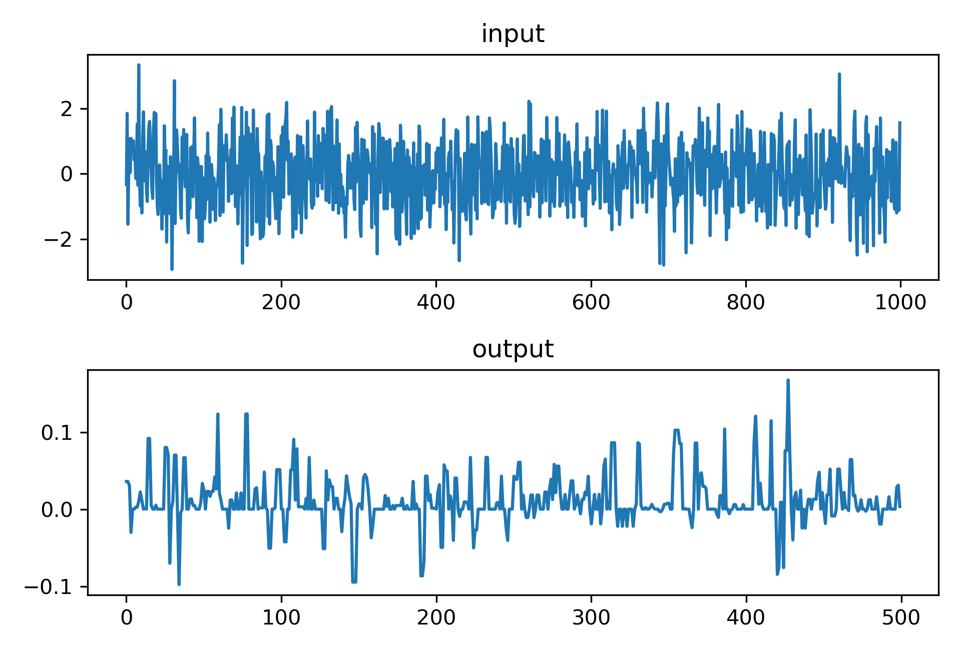
input = np.random.randn(1000)
output = pipe.feed(input) # the core, singular exposed method

# every other output will be a NaN to demarcate unready values
subsampled_output = output[1::pipe.stride]
That may be a lot to take in, so let me break it down for you:
rq.Pipeline(description...)constructs a filter pipeline from one or more filter descriptions and initializes internal state..feed(*)takes in a Python number ornp.arrayand its output is shaped likewise.- The two filter types are
rq.LowPassandrq.HighPassthat compute rolling quantiles and return them as is, and subtract them from the raw signal respectively. Compose them however you like! NaNs in the output purposefully indicate missing values, usually due to subsampling. If you pass aNaNinto aLowPassfilter, it will slowly deplete its reserve and continue to return valid quantiles until the window empties completely.rq.LowPassandrq.HighPassalternatively take in aquantile=qargument,0<=q<=1. The filters would perform a linear interpolation in this case. In order to control the statistical characteristics of this quantile estimate, parametersalphaandbetaare exposed as well with default values(1, 1). Refer to SciPy's documentation for details on this aspect.
interpolated_pipe = rq.Pipeline(
    # attempt to estimate the exact 40%-quantile by the
    # default linear interpolation with parameters (1, 1)
    rq.LowPass(window=30, quantile=0.4),
    # here, the estimate is "approximately unbiased" in
    # the case of Gaussian white noise
    rq.HighPass(window=10, quantile=0.3,
      alpha=3/8, beta=3/8))
See this Wikipedia section for an elucidating overview.
I also expose a convenience function rq.medfilt(signal, window_size) at the top-level of the package to directly supplant scipy.signal.medfilt.
That's it! I detailed the entire library. Don't let the size of its interface fool you!
If you are running Linux, MacOS, or Windows with Python 3.8+ and NumPy ~1.20, execute the following:
pip install rolling-quantiles
These are the conditions under which binaries are built and sent to the Python Package Index, which holds pip's packages. Should the NumPy version be unsuitable, for instance, I suggest building the package from source. This is rather straightforward because the handful of source files in C have absolutely minimal dependencies.
The meat of this package is a handful of C files with no external dependencies, besides NumPy 1.16+ and Python 3.7+ for the bindings located in src/python.c. As such, you may build from source by running the following from the project's root directory:
cd python- Check
pyproject.tomlto make sure the listed NumPy version matches your desired target. The compiled package will be forward- but not backward-compatible. python -m build(make sure this invokes Python 3)pip install dist/<name_of_generated_wheel_file>.whl
Make sure to specify MACOSX_DEPLOYMENT_TARGET=10.X as a prefix to the build command, e.g. python -m build. The placeholder X can be any MacOS version earlier than Big Sur (I use 9.) By default, the build system would attempt to build for MacOS 11 that is incompatible with current Python interpreters that have been compiled against a prior version.
I make use of binary heaps that impart desirable guarantees on their amortized runtime. Realistically, their performance may depend on the statistics of the incoming signal. I pummeled the filters with Gaussian Brownian motion to gauge their practical usability under a typical drifting stochastic process.
window |
rolling_quantiles [1] |
scipy [2] |
pandas [3] |
|---|---|---|---|
| 4 | 14 seconds | 22 seconds | 25 seconds |
| 10 | 21 seconds | 47 seconds | 31 seconds |
| 20 | 28 seconds | 95 seconds | 35 seconds |
| 30 | 30 seconds | 140 seconds | 37 seconds |
| 40 | 34 seconds | 190 seconds | 40 seconds |
| 50 | 36 seconds | 242 seconds | 40 seconds |
| 1,000 | 61 seconds | N/A | 62 seconds |
Likewise, with simulated Gaussian white noise (no drift in the signal):
window |
rolling_quantiles [1] |
scipy [2] |
pandas [3] |
|---|---|---|---|
| 4 | 14 seconds | 22 seconds | 25 seconds |
| 10 | 20 seconds | 51 seconds | 31 seconds |
| 20 | 25 seconds | 105 seconds | 36 seconds |
| 30 | 27 seconds | 156 seconds | 39 seconds |
| 40 | 30 seconds | 218 seconds | 41 seconds |
| 50 | 30 seconds | 279 seconds | 42 seconds |
| 1,000 | 45 seconds | N/A | 70 seconds |
Intel(R) Core(TM) i7-8700T CPU @ 2.40GHz, single-threaded performance on Linux. My algorithm looked even better (relative to pandas) on a 2020 MacBook Pro. Check out this StackOverflow answer for a particular use case.
[1] rq.Pipeline(...)
[2] scipy.signal.medfilt(...)
[3] pd.Series.rolling(*).quantile(...)
