This projects shares the same ROS Jetson configuration root file from: https://github.com/lmqZach/JetsonNano_PoseEstimation

The new algorithm for this progress file resides under root/navigation_dev/src

|-- ROOT
  |-- README.md
  |-- CMakeLists.txt
  |-- init.sh
  |-- jetbot_ROS
  |   |-- ```
  |-- jetson-inference
  |   |-- ```
  |-- navigation_dev
  |   |-- CMakeLists.txt
  |   |-- package.xml
  |   |-- launch
  |   |-- msg
  |   |-- src
  |          |-- april_detect.py
  |          |-- ekf.py
  |          |-- localization_node.py
  |          |-- planner_node.py
  |          |-- slam_node.py
  |-- ros_deep_learning
      |-- ```

The objective of this phase of project is to implement a version of the Simultaneous Localization and Mapping (SLAM) technique and evaluate its perfor- mance.

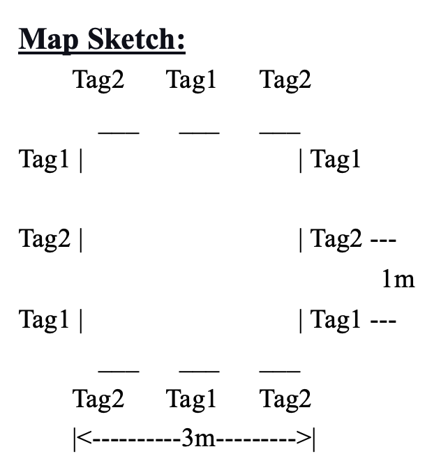
1. Setup an environment in a 10ft × 10ft area with landmarks as exemplified in the figure. The landmarks are 9 AprilTags in two types (Tag1 & Tag2) to represent natural objects.

2. Implement the KALMAN filter based SLAM system. Use the off-the-shelf software to detect the landmarks.

3. Drive through the environment to build up a map in two steps:

   i) Initially drive the robot in a circle

   ii) Drive through the environment using a figure 8 trajectory.

4. Compare the difference between the two generated maps.

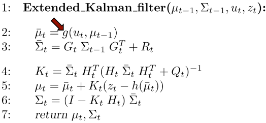
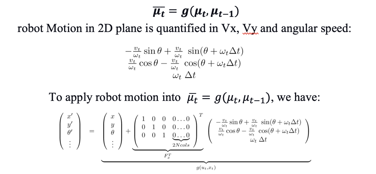
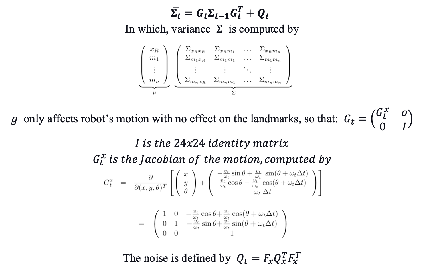
After achieving simple localization from the last assignment, this project focuses on constructing, updating the map of the test environment while recording Jetbot’s location by implementing Extended Kalman Filter (EKF). To apply EKF to our SLAM in the setup, we have divided the design logic into 5 parts: state prediction, measurement prediction, measurement, data association, and tag update.

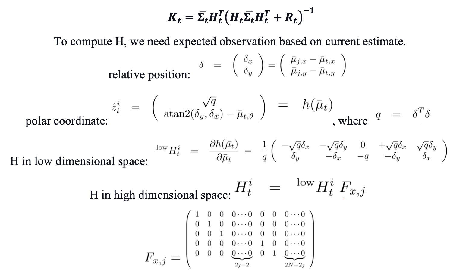
For every tag observed in a frame, we need to determine whether it is a new tag or not. If it is not a new tag, we also need to determine which tag it is associated with. We solved the problem by comparing the tag with all ‘seen’ tags in our estimated state vector. Specifically, for every tag in a frame, we computed its Euclidean distance in world coordinate to all seen tags in the same tag category (there are 2 tag categories in our setup). Then, we assigned the observation as a seen tag if the distance is less than a threshold. If no seen tags satisfied the condition, the algorithm would create a new tag and add the observation to our state vector. If the state vector is full, we then assign an observation to the tag with a minimum distance.

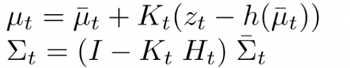
As what the purpose of Extended Kalman Filter should serve, the generated map plots after a few runs are better than the initial ones under circular motion, which verifies our implementation of the EKF to be effective. Tags are distinguished successfully in the sequence of blue and green which stands for ‘0’ and ‘42’ in our actual setup. Plot 1 can be interpreted as directly recognized tag positions due to the lack of EKF interference when there is only one circular motion. However, after two more circles, the EKF kicks in and corrects the tag positions more accurately to the actual environment. In addition, the X-Y coordinate of each tag is physically compared to the actual setup to make sure there is no significant difference. However, plot 3 under motion ‘8’ is less accurate than plot 1 and plot 2. Two tags in the same tag category are even detected which proofs the failure of the correction step. Plus, most tag positions are more away from the actual setup. In our general assumption, more complicated motion models does not suffice the Jetbot structure and the implementation of EKF.

The main constraint of this project is the accuracy of Jetbot’s motion model. Due to the simplicity of the robot motor and control magnetism, the motion model became the biggest barrier to better results. Proven in prior projects, the Jetbot has so much uncontrollable and unpredictable flexibility when completing specific motion commands. It leads to the discrepancy between our established motion model and the actual physical motion. Although efforts are made in noise calibration to make the trajectory as close as a circle, there are still a lot of inaccuracies. For example, we noticed the shift of the circle center during a continuous run, even after our best attempts to calibrate. Plus, there are other unnoticeable inaccuracies of the motion, which, altogether, causes noticeable difference from the predicted robot position. Under a more complicated motion, like number ‘8’, the discrepancy is even amplified and results in worse tag plots.

Other than using a more naturally ‘accurate’ robot, there are some potential adjustments that may help reduce the error. For instance, we could move the environment setup from carpet in the graduate common room to a smooth tiled floor. From our prior experience, surfaces with less friction tend to allow Jetbot motion to be closer to the command. However, this option is eliminated due to the size of the environment required for this setup. During calibration, we could use a marker pen attached to the robot during a run to physically ‘draw’ the trajectory. With the marker on the ground, we would have a better clue in predicting the error, and, as a result, change the noise matrix to achieve better results.

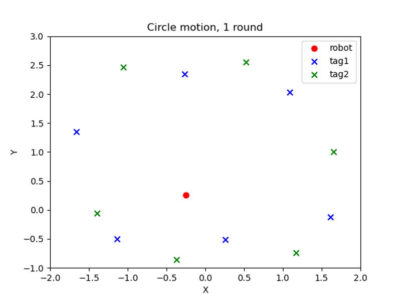
Figure 1: Map plot of circular motion, 1 round

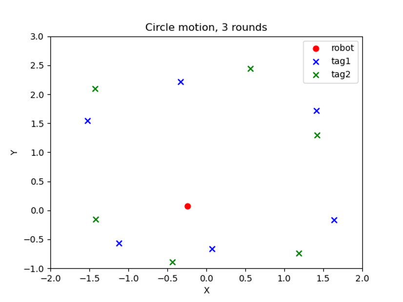
Figure 2: Map plot of circular motion, 3 rounds

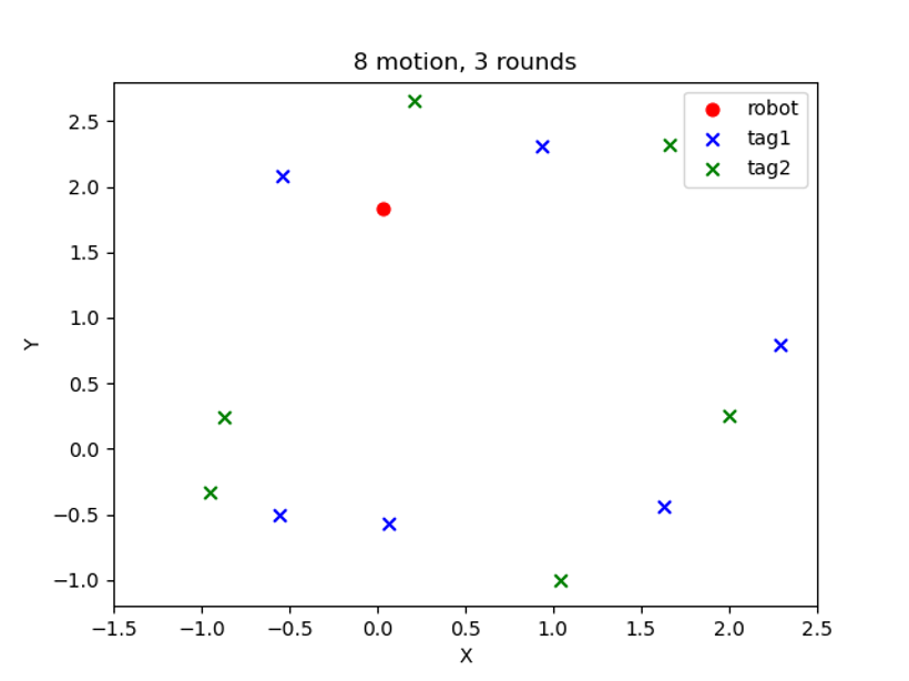
Figure 3: Map plot of number ‘8’ motion, 3 rounds