Data structure & algorithm using java
7 likes827 views

The document is a comprehensive guide to data structures and algorithms using Java, intended to help students understand and apply these concepts for developing applications and for job placement in tech companies. It includes foundational topics such as algorithms, data structures, sorting, searching techniques, and linked lists with practical examples and implementation details. Authored by Narayan Sau, the book aims to compile freely available information into a cohesive educational resource.


![Data Structure & Algorithm using Java
Page 18
Definiteness. Each step of an algorithm must be precisely defined down to the
last detail. The action to be carried out must be rigorously and unambiguously
specified for each case.
Input. An algorithm has zero or more inputs.
Output. An algorithm has one or more outputs.
Effectiveness. An algorithm is also generally expected to be effective in the
sense that its operations must all be sufficiently basic that they can in principle
be done exactly and in a finite length of time by someone using pencil and
paper.
Let us explain with an example. Consider the simplest problem of finding the G.C.D.
(H.C.F.) of two positive integer number m and n where n < m.
E1. [Find remainder.] Divide m by n and let r be the remainder. ( 0<=r<n)
E2. [Is it zero?] If r = 0, the algorithm terminates; n is the answer.
E3. [Reduce] Set m =n, n = r. go back to step E1.
The algorithm is terminating after finite number of steps [Finiteness]. All three steps
are precisely defined [Definiteness]. The actions carrying out are rigorous and
unambiguous. It has two [Input] and one [Output]. Also, the algorithm is effective in
the sense that its operations can be done in finite length of time [Effectiveness].
1.3 Role of a Data Structure
A problem can be solved with multiple algorithms. Therefore, we need to choose an
algorithm which provides maximum efficiency i.e. use minimum time and minimum
memory. Thus, data structures come into picture.
Data structure is the art of structuring the data in computer memory in such a
way that the resulting operations can be performed efficiently.
Data can be organized in many ways; therefore, you can create as many data
structures as you want. However, there are some standard data structures that have
proved to be useful over the years. These include arrays, linked lists, stacks, queues,
trees, and graphs. We will learn more about these data structures in the subsequent
sections. All these data structures are designed to hold a collection of data items.
However, the difference lies in the way the data items are arranged with respect to
each other and the operations that they allow. Because of the different ways in which
the data items are arranged with respect to each other, some data structures prove to
be more efficient than others in solving a given problem.](https://image.slidesharecdn.com/datastructurealgorithmusingjavav1-180530094707/85/Data-structure-algorithm-using-java-18-320.jpg)


![Data Structure & Algorithm using Java
Page 25
A new dynamic request for memory might return a range of addresses out of one of
the holes. But it might not use up the entire hole, so further dynamic requests might
be satisfied out of the original hole.
If too many small holes develop, memory is wasted because the total memory used
by the holes may be large, but the holes cannot be used to satisfy dynamic requests.
This situation is called memory fragmentation. Keeping track of allocated and de-
allocated memory is complicated. A modern operating system does all this.
Memory for an object can also be allocated dynamically during a method's execution,
by having that method utilize the special new operator built into Java. For example,
the following Java statement creates an array of integers whose size is given by the
value of variable k:
int[] items = new int[k];
The size of the array above is known only at runtime. Moreover, the array may continue
to exist even after the method that created it terminates. Thus, the memory for this
array cannot be allocated on the Java stack.
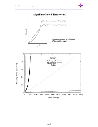
1.6 Algorithm Analysis
The analysis of algorithms is the determination of the computational complexity of
algorithms, i.e. the amount of time, storage and/or other resources necessary to
execute them. Usually, this involves determining a function that relates the length of
an algorithm's input to the number of steps it takes (its time complexity) or the number
of storage locations it uses (its space complexity).
An algorithm is said to be efficient when this function's values are small. Since different
inputs of the same length may cause the algorithm to have different behavior, the
function describing its performance is usually an upper bound on the actual
performance, determined from the worst case inputs to the algorithm.
A Priori Analysis− This is a theoretical analysis of an algorithm. Efficiency of
an algorithm is measured by assuming that all other factors, for example,
processor speed, are constant and have no effect on the implementation.
A Posterior Analysis− This is an empirical analysis of an algorithm. The
selected algorithm is implemented using programming language. This is then
executed on target computer machine. In this analysis, actual statistics like
running time and space required, are collected.
Time Factor− Time is measured by counting the number of key operations
such as comparisons in the sorting algorithm.
Space Factor− Space is measured by counting the maximum memory space
required by the algorithm.
In general, the running time of an algorithm or data structure method increases with
the input size, although it may also vary for different inputs of the same size. Also, the
running time is affected by the hardware environment (as reflected in the processor,
clock rate, memory, disk, etc.) and software environment (as reflected in the operating
system, programming language, compiler, interpreter, etc.) in which the algorithm is
implemented, compiled, and executed. All other factors being equal, the running time
of the same algorithm on the same input data will be smaller if the computer has, say,
a much faster processor or if the implementation is done in a program compiled into](https://image.slidesharecdn.com/datastructurealgorithmusingjavav1-180530094707/85/Data-structure-algorithm-using-java-25-320.jpg)


![Data Structure & Algorithm using Java
Page 34
1.8.1.3 Flexibility
Different implementations of an ADT, having all the same properties and abilities, are
equivalent and may be used somewhat interchangeably in code that uses the ADT.
This gives a great deal of flexibility when using ADT objects in different situations. For
example, different implementations of an ADT may be more efficient in different
situations; it is possible to use each in the situation where they are preferable, thus
increasing overall efficiency.
1.9 Arrays & Structure
Array is a fixed-size sequenced collection of variables belonging to the same data
types. The array has adjacent memory locations to store values.
An array data structure stores several elements of the same type in a specific order.
They are accessed using an integer to specify which element is required (although the
elements may be of almost any type). Arrays may be fixed-length or expandable.
When data objects are stored in an array, individual objects are selected by an index
that is usually a non-negative scalar integer. Indexes are also called subscripts. An
index maps the array value to a stored object.
There are three ways in which the elements of an array can be indexed:
0 (zero-based indexing): The first element of the array is indexed by subscript
of 0.
1 (one-based indexing): The first element of the array is indexed by subscript
of 1
n (n-based indexing): The base index of an array can be freely chosen. Usually
programming languages allowing n-based indexing, also allow negative index
values, and other scalar data types like enumerations, or characters may be
used as an array index.
1.9.1 Types of an Array
1.9.1.1 One-dimensional array
One-dimensional array (or single dimension array) is a type of linear array. Accessing
its elements involves a single subscript which can either represent a row or column
index.
Syntax:
DataType anArrayname[sizeofArray];
1.9.1.2 Multi-dimensional array
The number of indices needed to specify an element is called the dimension,
dimensionality, or rank of the array type.
This nomenclature conflicts with the concept of dimension in linear algebra, where it
is the number of elements. Thus, an array of numbers with 5 rows and 4 columns,
hence 20 elements, is said to have dimension 2 in computing contexts, but represents
a matrix with dimension 4 by 5 or 20 in mathematics. Also, the computer science
meaning of “rank” is similar to its meaning in tensor algebra but not to the linear algebra
concept of rank of a matrix.](https://image.slidesharecdn.com/datastructurealgorithmusingjavav1-180530094707/85/Data-structure-algorithm-using-java-34-320.jpg)
![Data Structure & Algorithm using Java
Page 35
There are some specific operations that can be performed or those that are supported
by the array. These are:
Traversing: It prints all the array elements one after another.
Inserting: It adds an element at given index.
Deleting: It is used to delete an element at given index.
Searching: It searches for an element(s) using given index or by value.
Updating: It is used to update an element at given index.
Resizing
Some languages allow dynamic arrays (also called resizable, growable, or extensible),
array variables whose index ranges may be expanded at any time after creation,
without changing the values of its current elements. For one-dimensional arrays, this
facility may be provided as an operation “append(A, x)” that increases the size of the
array A by one and then sets the value of the last element to x.
1.9.2 Array Declaration
In Java
int[] myIntArray = new int[3];
int[] myIntArray = {1,2,3};
int[] myIntArray = new int[]{1,2,3};
int[][] num = new int[5][2];
int num[][] = new int[5][2];
int[] num[] = new int[5][2];
1.9.3 Array Initialization
int[][] num = {{1,2}, {1,2}, {1,2}, {1,2}, {1,2}};
1.9.4 Memory allocation
1.9.5 Advantages & Disadvantages
1.9.5.1 Advantages
It is better and convenient way of storing the data of same data type with same size.
It allows us to store known number of elements in it.
It is used to represent multiple data items of same type by using only single name.
It can be used to implement other data structures like linked lists, stacks, queues,
trees, graphs etc. 2D arrays are used to represent matrices](https://image.slidesharecdn.com/datastructurealgorithmusingjavav1-180530094707/85/Data-structure-algorithm-using-java-35-320.jpg)


![Data Structure & Algorithm using Java
Page 38
2.2 Basic Operations
Stack operations may involve initializing the stack, using it, and then de-initializing it.
Apart from these basic stuffs, a stack is used for the following two primary operations−
push()− Pushing (storing) an element on the stack.
pop()− Removing (accessing) an element from the stack.
To use a stack efficiently, we need to check the status of stack as well. For the same
purpose, the following functionality is added to stacks−
top()− get the top data element of the stack, without removing it.
isFull()− check if stack is full. May not require for link list implementation.
isEmpty()− check if stack is empty.
At all times, we maintain a pointer to the last pushed data on the stack. As this pointer
always represents the top of the stack, hence it is named as top. The top pointer
provides top value of the stack without removing it.
2.2.1 peek()
Algorithm of peek() function–
begin procedure peek
return stack[top]
end procedure
2.2.2 isfull()
Algorithm of isfull() function–
begin procedure isfull
if top equals to MAXSIZE
return true
else
return false
endif
end procedure
2.2.3 isempty()
Algorithm of isempty() function–
Begin procedure isempty
if top less than 1
return true
else
return false
endif
end procedure
2.2.4 Push Operation
The process of putting a new data element onto stack is known as a Push Operation.
Push operation involves a series of steps−
Step 1− Checks if the stack is full.
Step 2− If the stack is full, produces an error and exit.
Step 3− If the stack is not full, increments top to point next empty space.](https://image.slidesharecdn.com/datastructurealgorithmusingjavav1-180530094707/85/Data-structure-algorithm-using-java-38-320.jpg)
![Data Structure & Algorithm using Java
Page 39
Step 4− Adds data element to the stack location, where top is pointing.
Step 5− Returns success.
If the linked list is used to implement the stack, then in step 3, we need to allocate
space dynamically.
2.2.4.1 Algorithm for Push Operation
A simple algorithm for Push operation can be derived as follows−
begin procedure push: stack, data
if stack is full
return null
endif
top ← top + 1
stack[top] ← data
end procedure
2.2.5 Pop Operation
Accessing the content while removing it from the stack is known as a Pop operation.
In an array implementation of pop() operation, the data element is not actually
removed, instead top is decremented to a lower position in the stack to point to the
next value. But in linked-list implementation, pop() actually removes data element and
deallocates memory space.
A Pop operation may involve the following steps−
Step 1− Checks if the stack is empty.
Step 2− If the stack is empty, produces an error and exit.
Step 3− If the stack is not empty, accesses the data element at which top is
pointing.
Step 4− Decreases the value of top by 1.
Step 5− Returns success.](https://image.slidesharecdn.com/datastructurealgorithmusingjavav1-180530094707/85/Data-structure-algorithm-using-java-39-320.jpg)
![Data Structure & Algorithm using Java
Page 40
2.2.5.1 Algorithm for Pop Operation
A simple algorithm for Pop operation can be derived as follows−
Begin procedure pop: stack
if stack is empty
return null
endif
data ← stack[top]
top ← top - 1
return data
end procedure
2.2.6 Program on stack link implementation
class Link<E>
{
// Singly linked list node
private E element; // Value for this node
private Link<E> next; // Pointer to next node in list
// Constructors
Link(E it, Link<E> nextval) {element = it; next = nextval;}
Link(Link<E> nextval) {next = nextval;}
Link<E> next() {return next;}
Link<E> setNext(Link<E> nextval) {return next = nextval;}
E element() {return element;}
E setElement(E it) {return element = it;}
} // class Link
class LStack <E> implements Stack <E> {
//class LStack<E> implements Stack<E> {
private Link<E> top; // Pointer to first element
private int size; // Number of elements
//Constructors
public LStack() {top = null; size = 0;}
public LStack(int size) {top = null; size = 0;}](https://image.slidesharecdn.com/datastructurealgorithmusingjavav1-180530094707/85/Data-structure-algorithm-using-java-40-320.jpg)
![Data Structure & Algorithm using Java
Page 41
// Reinitialize stack
public void clear() {top = null; size = 0;}
public void push(E it) { // Put “it” on stack
top = new Link<E>(it, top);
size++;
}
public E pop() { // Remove “it” from stack
assert top != null : “Stack is empty”;
E it = top.element();
top = top.next();
size--;
return it;
}
public E topValue() { // Return top value
assert top != null : “Stack is empty”;
return top.element();
}
public int length() {return size;} // Return length
@Override
public E top() {
// TODO Auto-generated method stub
return topValue();
}
@Override
public int size() {
// TODO Auto-generated method stub
return length();
}
@Override
public boolean isEmpty() {
// TODO Auto-generated method stub
return (size == 0) ;
}
public void display( ) {
String t;
if (isEmpty()) t = “Stack is Empty”; else t=“Stack has data”;
String s=“n[“ + t + “] Stack size:” + size + “Stack values[“;
Link<E> temp;
temp = top;
while (temp != null) {
s += temp.element();
if (temp.next ()!= null) s += “,” ;
temp = temp.next();
};
s += “]n”;
System.out.print(s);
}
}
public class StackLinkMain<E> {
public static void main (String[] args)
{
LStack <Integer> myStack = new LStack<Integer> ();](https://image.slidesharecdn.com/datastructurealgorithmusingjavav1-180530094707/85/Data-structure-algorithm-using-java-41-320.jpg)
![Data Structure & Algorithm using Java
Page 42
myStack.display();
for (int i = 1 ; i<10 ; i++)
myStack.push(i * i);
myStack.display();
myStack.pop();
myStack.display();
}
}
2.2.7 My Stack Array Implementation
/** Stack ADT */
public interface Stack<E> {
/** Reinitialize the stack. The user is responsible for
reclaiming the storage used by the stack elements. */
public void clear();
/** Push an element onto the top of the stack.
@param it The element being pushed onto the stack. */
public void push(E it);
/** Remove and return the element at the top of the stack.
@return The element at the top of the stack. */
public E pop() ;
// Return TOP element
public E top() ;
/** @return A copy of the top element. */
public E topValue();
/** @return The number of elements in the stack. */
public int size();
// Check if the stack is empty
public boolean isEmpty();
};
public class arrayStack<E> implements Stack<E> {
private E[] listStack; // Array holding list elements
private static final int MAXSIZE = 10; // Maximum size of list
private int top; // Number of list items now
public arrayStack() {top = 0;}
public void arrayStackfill (E[] listArray) {
this.listStack = listArray;
}
@Override
public void clear() {top = 0;}
@Override
public void push(E it) {
// TODO Auto-generated method stub
if (top == MAXSIZE)
System.out.println(“Stack is full n”);
listStack[top++] = it;
}
@Override
public E pop() {
// TODO Auto-generated method stub
if (top == 0) return null;](https://image.slidesharecdn.com/datastructurealgorithmusingjavav1-180530094707/85/Data-structure-algorithm-using-java-42-320.jpg)
![Data Structure & Algorithm using Java
Page 43
System.out.println(“top Value : “ +
listStack[top - 1] + “ is getting poped”);
return (listStack[top--]);
}
@Override
public E top() {
// TODO Auto-generated method stub
if (top == 0)
return null;
System.out.println(“Top of the stack is : “ + size() +
“ And Value : “ + listStack[top - 1]);
return (listStack[top - 1]);
}
@Override
public E topValue() {
// TODO Auto-generated method stub
return top();
}
@Override
public int size() {
// TODO Auto-generated method stub
return top;
}
@Override
public boolean isEmpty() {
// TODO Auto-generated method stub
return (top == 0);
}
public void display( ) {
String t;
if (isEmpty()) t = “ Stack is Empty” ;
else t = “Stack has data”;
String s = “n[ “ + t + “ ] Stack size :” + size() +
“ Stack values [ “;
for (int i = top - 1; i>= 0; i--) {
s += listStack[i] ;
s += “,” ;
}
s += “]n”;
System.out.print(s);
}
}
public class arrayStackImpl {
public static void main(String[] args) {
// TODO Auto-generated method stub
//int [] listArray;
Integer[] listArray = {1,1,1,1,1,1,1,1,1,1};
arrayStack<Integer > myStack = new arrayStack<Integer> ();
System.out.println(“Stack is started n”);
myStack.arrayStackfill(listArray);
//myStack.display();
myStack.clear();
myStack.display();
myStack.push(10);
for (int i = 1; i<8; i++)](https://image.slidesharecdn.com/datastructurealgorithmusingjavav1-180530094707/85/Data-structure-algorithm-using-java-43-320.jpg)


![Data Structure & Algorithm using Java
Page 47
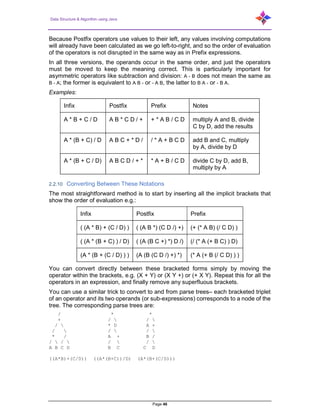
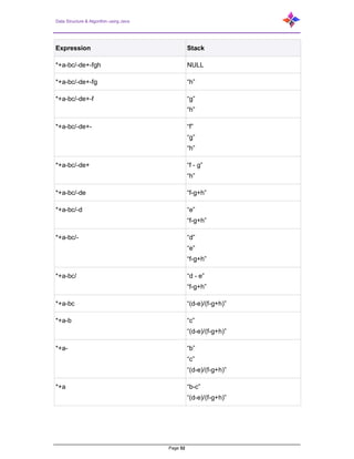
2.2.11 Infix to Postfix using Stack
Let X be an arithmetic expression written in infix notation. This algorithm finds the
equivalent postfix expression Y.
Push “(“onto Stack, and add “)” to the end of X.
Scan X from left to right and repeat Step 3 to 6 for each element of X until the
Stack is empty.
If an operand is encountered, add it to Y.
If a left parenthesis is encountered, push it onto Stack.
If an operator is encountered, then:
Repeatedly pop from Stack and add to Y each operator (on the top of
Stack) which has the same precedence as or higher precedence than
operator.
Add operator to Stack.
[End of If]
If a right parenthesis is encountered, then:
Repeatedly pop from Stack and add to Y each operator (on the top of
Stack) until a left parenthesis is encountered.
Remove the left Parenthesis.
[End of If]
END.
Let’s take an example to better understand the algorithm.
Infix Expression: A+(B*C-(D/E^F)*G)*H, where ^ is an exponential operator.](https://image.slidesharecdn.com/datastructurealgorithmusingjavav1-180530094707/85/Data-structure-algorithm-using-java-47-320.jpg)

![Data Structure & Algorithm using Java
Page 49
2) Read postfix expression Left to Right until ) encountered
3) If operand is encountered, push it onto Stack
[End If]
4) If operator is encountered, Pop two elements
i) A -> Top element
ii) B-> Next to Top element
iii) Evaluate B operator A
iv) Push B operator A onto Stack
5) Set result = pop
6) END
Let's see an example to better understand the algorithm:
Expression: 456*+](https://image.slidesharecdn.com/datastructurealgorithmusingjavav1-180530094707/85/Data-structure-algorithm-using-java-49-320.jpg)


![Data Structure & Algorithm using Java
Page 56
A real-world example of queue can be a single-lane one-way road, where the vehicle
that enters first, exits first. More real-world examples can be seen as queues at the
ticket windows and bus-stops.
3.3 Queue Representation
As we now understand that in queue, we access both ends for different reasons. The
following diagram tries to explain queue representation as data structure−
As in stacks, a queue can also be implemented using Arrays, Linked-lists, Pointers
and Structures. For the sake of simplicity, we shall implement queues using one-
dimensional array.
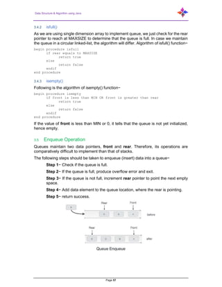
3.4 Basic Operations
Queue operations may involve initializing or defining the queue, utilizing it, and then
completely erasing it from the memory. Here we shall try to understand the basic
operations associated with queues–
Mainly the following basic operations are performed on queue:
Enqueue: Adds an item to the queue. If the queue is full, then it is said to be
an Overflow condition.
Dequeue: Removes an item from the queue. The items are popped in the same
order in which they are pushed. If the queue is empty, then it is said to be an
Underflow condition.
Rear: Get the last item from queue.
Front(), peek()− Gets the element at the front of the queue without removing
it.
isfull()− Checks if the queue is full.
isempty()− Checks if the queue is empty.
In queue, we always dequeue (or access) data, pointed by front pointer and while
enqueuing (or storing) data in the queue we take help of rear pointer.
Let's first learn about supportive functions of a queue.
3.4.1 peek()
This function helps to see the data at the front of the queue. The algorithm of peek()
function is as follows−
begin procedure peek
return queue[front]
end procedure](https://image.slidesharecdn.com/datastructurealgorithmusingjavav1-180530094707/85/Data-structure-algorithm-using-java-56-320.jpg)
![Data Structure & Algorithm using Java
Page 58
Sometimes we also check to see if a queue is initialized or not, to handle any
unforeseen situations.
Algorithm for enqueue operation−
begin procedure enqueue(data)
if queue is full
return overflow
endif
rear ← rear + 1
queue[rear] ← data
return true
end procedure
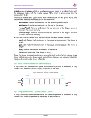
3.6 Dequeue Operation
Accessing data from the queue is a process of two tasks− access the data where front
is pointing, and remove the data after access. The following steps are taken to perform
dequeue operation−
Step 1− Check if the queue is empty.
Step 2− If the queue is empty, produce underflow error and exit.
Step 3− If the queue is not empty, access the data where front is pointing.
Step 4− Increment front pointer to point to the next available data element.
Step 5− Return success.
Algorithm for dequeue operation
begin procedure dequeue
if queue is empty
return underflow
end if
data = queue[front]
front ← front + 1
return true
end procedure
3.7 Queue using Linked List
The major problem with a queue implemented using array is that it works for only fixed
number of data. That amount of data must be specified in the beginning itself. Queue](https://image.slidesharecdn.com/datastructurealgorithmusingjavav1-180530094707/85/Data-structure-algorithm-using-java-58-320.jpg)

![Data Structure & Algorithm using Java
Page 60
Step 4: Then set 'front = front → next' and delete 'temp' (free(temp)).
3.8.3 display()– Displaying the elements of Queue
We can use the following steps to display the elements (nodes) of a queue.
Step 1: Check whether queue is Empty (front == NULL).
Step 2: If it is Empty then, display message 'Queue is empty' and terminate
the function.
Step 3: If it is Not Empty then, define a Node pointer 'temp' and initialize with
front.
Step 4: Display 'temp → data --->' and move it to the next node. Repeat the
same until 'temp' reaches to 'rear' (temp → next != NULL).
Step 5: Finally! Display 'temp → data ---> NULL'.
3.8.3.1 Abstract Data Type definition of Queue/Dequeue
/** Queue ADT My program */
public interface Queue<E> {
/** Reinitialize the queue. The user is responsible for
Reclaiming the storage used by the queue elements. */
public void clear();
/** Place an element at the rear of the queue.
@param it The element being enqueued. */
public void enqueue(E it);
/** Remove and return element at the front of the queue.
@return the element at the front of the queue. */
public E dequeue();
/** @return the front element. */
public E peek();
/** @return the number of elements in the queue. */
public int length();
//Checks if the queue is full.
public boolean isFull();
// Checks if the queue is empty.
public boolean isEmpty();
}
package ADTList;
public class arrayQueue <E> implements Queue<E> {
private E[] listQueue; // Array holding list elements
private static final int MAXSIZE = 10; // Maximum size of list
private int front, rear, size; // Number of list items now
//Constructor
public arrayQueue () {
front = size = 0;
rear = -1;
//for (int i = 0 ; i< MAXSIZE ; i++) listQueue[i] = null;
}](https://image.slidesharecdn.com/datastructurealgorithmusingjavav1-180530094707/85/Data-structure-algorithm-using-java-60-320.jpg)
![Data Structure & Algorithm using Java
Page 61
@Override
public void clear() {
// TODO Auto-generated method stub
front = size = 0;
rear = -1;
for (int i = 0 ; i< MAXSIZE ; i++) listQueue[i] = null;
return;
}
@Override
public void enqueue(E it) {
// TODO Auto-generated method stub
if (size == MAXSIZE) return;
rear++;
listQueue[rear] = it;
size++;
}
@Override
public E dequeue () {
// TODO Auto-generated method stub
if (front > rear) return null ;
size--;
return (listQueue[front++]);
}
public E frontValue() {
// TODO Auto-generated method stub
return (listQueue[front]);
}
@Override
public int length() {
// TODO Auto-generated method stub
return (size);
}
@Override
public E peek() {
// TODO Auto-generated method stub
return frontValue();
}
@Override
public boolean isFull() {
// TODO Auto-generated method stub
return (rear == MAXSIZE) ;
}
@Override
public boolean isEmpty() {
// TODO Auto-generated method stub
R return ((rear - front)<=0);
}
public void arrayQueuefill (E[] listArray) {
this.listQueue= listArray;
}
public void display( ) {](https://image.slidesharecdn.com/datastructurealgorithmusingjavav1-180530094707/85/Data-structure-algorithm-using-java-61-320.jpg)
![Data Structure & Algorithm using Java
Page 62
String t;
if (isEmpty()) t = “Queue is Empty”; else t = “Queue has data”;
String s = “n[ “ + t + “ ] Queue size :” +
size + “ Queue values [ “;
for (int i = front; i <= size; i++) {
s += listQueue[i] ;
s += “,” ;
}
s += “]n”;
System.out.print(s);
}
}
/**
*** @author Narayan
**/
public class arrayQueueImpl {
/**
* @param args
*/
public static void main(String[] args) {
// TODO Auto-generated method stub
arrayQueue<Integer> myQueue = new arrayQueue<Integer> ();
Integer[] listQueue = {0,1,1,1,1,1,1,1,1,1};
System.out.println(“Queue is startedn”);
myQueue.arrayQueuefill(listQueue);
myQueue.display();
for (int i = 1; i<8 ; i++) myQueue.enqueue(i*i);
myQueue.display();
myQueue.dequeue();
myQueue.display();
myQueue.clear();
myQueue.display();
}
}
3.8.3.2 Linked List implementation of Queue
/** Queue ADT */
public interface Queue<E> {
/** Reinitialize the queue. The user is responsible for
reclaiming the storage used by the queue elements. */
public void clear();
/** Place an element at the rear of the queue.
@param it The element being enqueued. */
public void enqueue(E it);
/** Remove and return element at the front of the queue.
@return The element at the front of the queue. */
public E dequeue();
/** @return The front element. */
public E peek();
/** @return The number of elements in the queue. */
public int length();
//Checks if the queue is full.
public boolean isFull();](https://image.slidesharecdn.com/datastructurealgorithmusingjavav1-180530094707/85/Data-structure-algorithm-using-java-62-320.jpg)

![Data Structure & Algorithm using Java
Page 64
public boolean isEmpty() {
// TODO Auto-generated method stub
return (size == 0);
}
public void display( ) {
String t;
if (isEmpty()) t = “ Queue is Empty” ;
else t = “Queue has data “;
String s = “n[ “ + t + “ ] Queue size :” +
length() + “ Queue values [ “;
Link<E> temp;
temp = front;
while (temp != null) {
s += temp.element();
if (temp.next() != null) s += “,” ;
temp = temp.next();
} ;
s += “] front element : “ ;
s += peek();
s += “n”;
System.out.print(s);
}
}
package ADTList;
/**
* @author Narayan
*
**/
public class QueueLinkMain<E> {
public static void main (string[] args) {
LQueue <Integer> myQueue = new LQueue<Integer> ();
myQueue.display();
myQueue.enqueue(5);
myQueue.display();
for (int i = 1 ; i<10 ; i++)
myQueue.enqueue(i * i);
myQueue.display();
myQueue.dequeue(); myQueue.dequeue();
//myQueue.pop();
myQueue.display();
}
}
[Queue is empty] Queue size: 0, Queue values [ ] front element: null
[Queue has data] Queue size: 1, Queue values [5] front element: 5
[Queue has data] Queue size: 10, Queue values [5,1,4,9,16,25,36,49,64,81], front
element: 5
[Queue has data] Queue size: 8, Queue values [4,9,16,25,36,49,64,81], front element:
4
3.9 Deque
Consider now a queue-like data structure that supports insertion and deletion at both
the front and the rear of the queue. Such an extension of a queue is called a double-](https://image.slidesharecdn.com/datastructurealgorithmusingjavav1-180530094707/85/Data-structure-algorithm-using-java-64-320.jpg)

![Data Structure & Algorithm using Java
Page 69
* // header.next().next().setPrev(header) ;
* // header.setNext(header.next().next());
* if you set Next first then code is as follows
*****************************************************/
header.setNext(header.next().next());
header.next().setPrev(header) ;
size--;
return (it);
}
@Override
public E removeLast() {
// TODO Auto-generated method stub
if (size == 0) {
System.out.println(“The D Q is empty : “);
return null;
}
E it = trailer.prev().element();
System.out.println(“removing last : “ + it);
trailer.setPrev(trailer.prev().prev());
trailer.prev().setNext(trailer);
size--;
return (it);
}
public void display() {
String t;
if (isEmpty()) t = “D-Q is Empty” ; else t = “D-Q has data“;
String s = “n[ “ + t + “ ] D-Q size:” + size + “ D-Q values [“;
DoublyLink <E> temp ;
temp = header.next();
while (temp != null)
{
if (temp.element() != null) s += temp.element() + “, “;
temp = temp.next();
} ;
s += “] “ ;
s += “n”;
System.out.print(s);
}
}
package ADTList;
/**
* @author Narayan
*
*/
public class DQueImplementMain {
/**
* @param args
*/
public static void main(String[] args) {
// TODO Auto-generated method stub
DQueuImplement <Integer> myDQue =
new DQueuImplement <Integer> ();
myDQue.display();
myDQue.addLast(500);](https://image.slidesharecdn.com/datastructurealgorithmusingjavav1-180530094707/85/Data-structure-algorithm-using-java-69-320.jpg)
![Data Structure & Algorithm using Java
Page 70
myDQue.addFirst(5);
myDQue.display();
myDQue.addFirst(10);
myDQue.addLast(50);
myDQue.display();
myDQue.getFirst();
myDQue.getLast();
myDQue.removeFirst();
myDQue.removeLast();
myDQue.display();
}
}
Console:
[D-Q is Empty] D-Q size: 0, D-Q values [ ]
[D-Q has data] D-Q size: 2, D-Q values [5, 500,]
[D-Q has data] D-Q size: 4, D-Q values [10, 5, 500, 50,]
First Element: 10
Last Element: 50
removing fast: 10
removing last: 50
[D-Q has data] D-Q size: 2, D-Q values [5, 500,]
3.12 Circular Queue
In a normal Queue data structure, we can insert elements until queue becomes full.
But once queue becomes full, we cannot insert the next element until all the elements
are deleted from the queue. For example, consider the queue below.
After inserting all the elements into the queue.
Now consider the following situation after deleting three elements from the queue.
This situation also says that Queue is full and we cannot insert the new element
because, 'rear' is still at last position. In above situation, even though we have empty
positions in the queue we cannot make use of them to insert new element. This is the
major problem in normal queue data structure. To overcome this problem, we use
circular queue data structure.](https://image.slidesharecdn.com/datastructurealgorithmusingjavav1-180530094707/85/Data-structure-algorithm-using-java-70-320.jpg)
![Data Structure & Algorithm using Java
Page 71
A Circular Queue can be defined as follows:
Circular Queue is a linear data structure in which the operations are performed
based on FIFO (First in First Out) principle and the last position is connected
back to the first position to make a circle.
Graphical representation of a circular queue is as follows:
3.12.1 Implementation of Circular Queue
To implement a circular queue data structure using array, we first perform the following
steps before we implement actual operations.
Step 1: Include all the header files which are used in the program and define
a constant 'SIZE' with specific value.
Step 2: Declare all user defined functions used in circular queue
implementation.
Step 3: Create a one-dimensional array with above defined SIZE (int
cQueue[SIZE])
Step 4: Define two integer variables 'front' and 'rear' and initialize both with
'-1'. (int front = -1, rear = -1)
Step 5: Implement main method by displaying menu of operations list and make
suitable function calls to perform operation selected by the user on circular
queue.
3.12.2 enQueue(value) - Inserting value into the Circular Queue
In a circular queue, enQueue() is a function which is used to insert an element into the
circular queue. In a circular queue, the new element is always inserted at rear position.
The enQueue() function takes one integer value as parameter and inserts that value
into the circular queue. We can use the following steps to insert an element into the
circular queue.
Step 1: Check whether queue is FULL. ((rear == SIZE-1 && front == 0) ||
(front == rear+1))
Step 2: If it is FULL, then display message “Queue is FULL. Insertion is not
possible” and terminate the function.
Step 3: If it is NOT FULL, then check rear == SIZE - 1 && front != 0 if it is
TRUE, then set rear = -1.
Step 4: Increment rear value by one (rear++), set queue[rear] = value and
check 'front == -1' if it is TRUE, then set front = 0.](https://image.slidesharecdn.com/datastructurealgorithmusingjavav1-180530094707/85/Data-structure-algorithm-using-java-71-320.jpg)
![Data Structure & Algorithm using Java
Page 72
3.12.3 deQueue()– Deleting a value from the Circular Queue
In a circular queue, deQueue() is a function used to delete an element from the circular
queue. In a circular queue, the element is always deleted from front position. The
deQueue() function doesn't take any value as parameter. We can use the following
steps to delete an element from the circular queue...
Step 1: Check whether queue is EMPTY (front == -1 && rear == -1)
Step 2: If it is EMPTY, then display message “Queue is EMPTY. Deletion is
not possible” and terminate the function.
Step 3: If it is NOT EMPTY, then display queue[front] as deleted element and
increment the front value by one (front++). Then check whether front == SIZE,
if it is TRUE, then set front = 0. Then check whether both front - 1 and rear
are equal (front -1 == rear), if it is TRUE, then set both front and rear to '-1'
(front = rear = -1).
3.12.4 display()– Displays the elements of a Circular Queue
We can use the following steps to display the elements of a circular queue...
Step 1: Check whether queue is EMPTY. (front == -1)
Step 2: If it is EMPTY, then display message “Queue is EMPTY” and
terminate the function.
Step 3: If it is NOT EMPTY, then define an integer variable 'i' and set 'i = front'.
Step 4: Check whether 'front <= rear', if it is TRUE, then display 'queue[i]'
value and increment 'i' value by one (i++). Repeat the same until 'i <= rear'
becomes FALSE.
Step 5: If 'front <= rear' is FALSE, then display 'queue[i]' value and increment
'i' value by one (i++). Repeat the same until' i <= SIZE - 1' becomes FALSE.
Step 6: Set i to 0.
Step 7: Again display 'cQueue[i]' value and increment i value by one (i++).
Repeat the same until 'i <= rear' becomes FALSE.
3.13 Priority Queue
Priority queues are a generalization of stacks and queues. Rather than inserting and
deleting elements in a fixed order, each element is assigned a priority represented by
an integer. We always remove an element with the highest priority, which is given by
the minimal integer priority assigned. Priority queues often have a fixed size.
For example, in an operating system the runnable processes might be stored in a
priority queue, where certain system processes are given a higher priority than user
processes. Similarly, in a network router packets may be routed according to some
assigned priorities. In both examples, bounding the size of the queues helps to prevent
so-called denial-of-service attacks where a system is essentially disabled by flooding
its task store. This can happen accidentally or on purpose by a malicious attacker.
A Priority Queue is an abstract data structure for storing a collection of
prioritized elements](https://image.slidesharecdn.com/datastructurealgorithmusingjavav1-180530094707/85/Data-structure-algorithm-using-java-72-320.jpg)


![Data Structure & Algorithm using Java
Page 75
public String getJob() {
return job;
}
/**
* @param job the job to set
*/
public void setJob(String job) {
this.job = job;
}
/**
* @return the priority
*/
public int getPriority() {
return priority;
}
/**
* @param priority the priority to set
*/
public void setPriority(int priority) {
this.priority = priority;
}
/* (non-Javadoc)
* @see java.lang.Object#toString()
*/
@Override
public String toString() {
return “Task [job=“ + job + “, priority=“ + priority + “]”;
}
}
package ADTList;
/**
* @author Narayan
*
*/
public class PriorityQueueWithTask {
private Task[] heap;
private int heapSize, capacity;
/**
* @param capacity
**/
public PriorityQueueWithTask(int capacity) {
this.capacity = capacity + 1;
heap = new Task[this.capacity];
heapSize = 0;
}
public void clear() {
heap = new Task[capacity];
heapSize = 0;
}
public boolean isEmpty() {return heapSize ==0;}
public boolean isFull() {return heapSize == (capacity - 1);}](https://image.slidesharecdn.com/datastructurealgorithmusingjavav1-180530094707/85/Data-structure-algorithm-using-java-75-320.jpg)
![Data Structure & Algorithm using Java
Page 76
/**
* @return the heapSize
**/
public int getHeapSize() {
return heapSize;
}
public void insert (String job, int priority) {
Task newJob = new Task(job, priority);
heap[++heapSize] = newJob;
int pos = heapSize;
while (pos != 1 && newJob.priority > heap[pos/2].priority) {
heap[pos] = heap[pos/2];
pos /= 2;
}
heap[pos] = newJob;
System.out.println(“[ Inserted ] “ + newJob.toString());
}
/** function to remove task **/
public Task remove() {
int parent, child;
Task item, temp;
if (isEmpty()) {
System.out.println(“Heap is empty”);
return null;
}
item = heap[1];
temp = heap[heapSize--];
parent = 1;
child = 2;
while (child <= heapSize) {
if (child < heapSize && heap[child].priority
< heap[child + 1].priority)
child++;
if (temp.priority >= heap[child].priority)
break;
heap[parent] = heap[child];
parent = child;
child *= 2;
}
heap[parent] = temp;
System.out.println(“[Removed: ] “ + temp.toString());
return item;
}
}
package ADTList;
/**
* @author Narayan
*
*/
public class myPriorityQueueTest {
/**
* @param args
*/
public static void main(String[] args) {
// TODO Auto-generated method stub
System.out.println(“Priority Queue Testn”);
System.out.println(“Enter size of priority queue “);](https://image.slidesharecdn.com/datastructurealgorithmusingjavav1-180530094707/85/Data-structure-algorithm-using-java-76-320.jpg)
![Data Structure & Algorithm using Java
Page 77
PriorityQueueWithTask pq = new PriorityQueueWithTask(30);
for (int i = 1 ; i < 9 ; i++) {
String s= “My Job no:” + i ;
pq.insert(s, i*i);
}
pq.remove();
}
}
3.15 Adaptable Priority Queues
There are situations where additional methods would be useful, as shown in the
scenarios below, which refer to a standby airline passenger application.
A standby passenger with a pessimistic attitude may become tired of waiting
and decide to leave ahead of the boarding time, requesting to be removed from
the waiting list. Thus, we would like to remove from the priority queue the entry
associated with this passenger. Operation removeMin is not suitable for this
purpose since the passenger leaving is unlikely to have first priority. Instead,
we would like to have a new operation remove (e) that removes an arbitrary
entry e.
Another standby passenger finds her gold frequent-flyer card and shows it to
the agent. Thus, her priority must be modified accordingly. To achieve this
change of priority, we would like to have a new operation replaceKey(e, k) that
replaces with k the key of entry e in the priority queue.
Finally, a third standby passenger notices her name is misspelled on the ticket
and asks it to be corrected. To perform the change, we need to update the
passenger's record. Hence, we would like to have a new operation
replaceValue(e, x) that replaces with x the value of entry e in the priority queue.
3.16 Multiple Queues
We have discussed efficient implementation of k stack in an array. In this section, same
for queue is discussed. Following is the detailed problem statement.
Create a data structure kQueues that represents k queues. Implementation of
kQueues should use only one array, i.e., k queues should use the same array
for storing elements. Following functions must be supported by kQueues.
enqueue(int x, int qn)–> adds x to queue number ‘qn’ where qn is from 0 to k-1
dequeue(int qn)–> deletes an element from queue number ‘qn’ where qn is from
0 to k-1
3.16.1 Method 1: Divide the array in slots of size n/k
A simple way to implement k queues is to divide the array in k slots of size n/k each,
and fix the slots for different queues, i.e., use arr[0] to arr[n/k-1] for first queue, and
arr[n/k] to arr[2n/k-1] for queue2 where arr[] is the array to be used to implement two
queues and size of array be n.
The problem with this method is inefficient use of array space. An enqueue operation
may result in overflow even if there is space available in arr[]. For example, consider
k as 2 and array size n as 6. Let us enqueue 3 elements to first and do not enqueue](https://image.slidesharecdn.com/datastructurealgorithmusingjavav1-180530094707/85/Data-structure-algorithm-using-java-77-320.jpg)
![Data Structure & Algorithm using Java
Page 78
anything to second queue. When we enqueue 4th element to first queue, there will be
overflow even if we have space for 3 more elements in array.
3.16.2 Method 2: A space efficient implementation
The idea is similar to the stack post. Here we need to use three extra arrays. In stack
post, we needed two extra arrays, one more array is required because in queues,
enqueue() and dequeue() operations are done at different ends.
Following are the three extra arrays are used:
front[]: This is of size k and stores indexes of front elements in all queues.
rear[]: This is of size k and stores indexes of rear elements in all queues.
next[]: This is of size n and stores indexes of next item for all items in array
arr[]. Here arr[] is actual array that stores k stacks.
Together with k queues, a stack of free slots in arr[] is also maintained. The top of this
stack is stored in a variable ‘free’.
All entries in front[] are initialized as -1 to indicate that all queues are empty. All entries
next[i] are initialized as i+1 because all slots are free initially and pointing to next slot.
Top of free stack, ‘free’ is initialized as 0.
3.17 Applications of Queue Data Structure
Queues are used for any situation where you want to efficiently maintain a first-in-first
out order on some entities. These situations arise literally in every type of software
development.
Imagine you have a web-site which serves files to thousands of users. You cannot
service all requests, you can only handle say 100 at once. A fair policy would be first-
come-first serve: serve 100 at a time in order of arrival. A Queue would be the most
appropriate data structure.
Similarly, in a multitasking operating system, the CPU cannot run all jobs at once, so
jobs must be batched up and then scheduled according to some policy. Again, a queue
might be a suitable option in this case.
Stacks are used for the undo buttons in various software. The recent most changes
are pushed into the stack. Even the back button on the browser works with the help of
the stack where all the recently visited web pages are pushed into the stack.
Queues are used in case of printers or uploading images where the first one to be
entered is the first to be processed.
3.18 Applications of Stack
Parsing in a compiler.
Java virtual machine.
Undo in a word processor.
Back button in a Web browser.
PostScript language for printers.
Implementing function calls in a compiler.](https://image.slidesharecdn.com/datastructurealgorithmusingjavav1-180530094707/85/Data-structure-algorithm-using-java-78-320.jpg)

![Data Structure & Algorithm using Java
Page 81
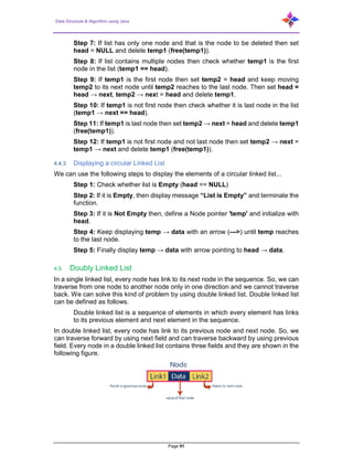
4 Linked List
Simply, a list is a sequence of data, and linked list is a sequence of data linked with
each other.
Like arrays, Linked List is a linear data structure. Unlike arrays, linked list elements
are not stored at contiguous location; the elements are linked using pointers.
4.1 Why Linked List?
Arrays can be used to store linear data of similar types, but arrays have following
limitations.
The size of the arrays is fixed. So, we must know the upper limit on the number
of elements in advance. Also, generally, the allocated memory is equal to the
upper limit irrespective of the usage.
Inserting a new element in middle of an array of elements is expensive;
because room must be created for the new elements and to create room
existing elements must shift.
For example, in a system if we maintain a sorted list of IDs in an array id[].
id[] = [1000, 1010, 1050, 2000, 2040]
And if we want to insert a new ID 1005, then to maintain the sorted order, we must
move all the elements after 1000 (excluding 1000).
Deletion is also expensive with arrays until unless some special techniques are used.
For example, to delete 1010 in id[], everything after 1010 must be moved.
Advantages of Linked List over Arrays:
Dynamic size
Ease of insertion/deletion
Drawbacks:
Random access is not allowed. We have to access elements sequentially
starting from the first node. So, we cannot do binary search with linked lists.
Extra memory space for a pointer is required with each element of the list.
4.2 Singly Linked List
In a singly linked list, each node in the list stores the contents of the node and a pointer
or reference to the next node in the list. It does not store any pointer or reference to
the previous node. It is called a singly linked list because each node only has a single
link to another node. To store a single linked list, you only need to store a reference](https://image.slidesharecdn.com/datastructurealgorithmusingjavav1-180530094707/85/Data-structure-algorithm-using-java-81-320.jpg)


![Data Structure & Algorithm using Java
Page 86
public myNode Search(myNode node, int da) {
myNode temp;
temp = node;
while (temp != null) {
if (temp.getData() == da) return temp;
temp = temp.next;
}
System.out.println(“n” + da + “ : not found “);
return temp;
}
public myNode SearchAndPointPrev(myNode node, int da) {
myNode temp, prev;
temp = node;
prev = node;
while (temp != null) {
if (temp.getData() == da) {
System.out.println(“n” + “ : data found... “);
return prev;
}
prev = temp;
temp = temp.next;
}
System.out.println(“n” + da + “ : not found “);
return prev;
}
public void Display(myNode node) {
myNode temp;
temp = node;
System.out.println(“n”);
while (temp != null) {
System.out.print(“ { “ + temp.getData() + “} --> “);
temp = temp.next;
}
System.out.print(“{null}”);
}
public static void main(String args[]) {
myNode linklist = new myNode();
myNode head, mydata;
head = linklist;
linklist.setData(5);
linklist.setNext(null);
linklist.Display(head);
for (int i = 1 ; i <10 ; i++) {
mydata = new myNode(i*i, null);
linklist.next = mydata;
linklist = mydata;
head.Display(head);
}
// find a particular node and insert data after that.
myNode temp;
temp = head.Search(head, 36);
if (temp != null)](https://image.slidesharecdn.com/datastructurealgorithmusingjavav1-180530094707/85/Data-structure-algorithm-using-java-86-320.jpg)


![Data Structure & Algorithm using Java
Page 97
// Move down list to “pos” position
public void moveToPos(int pos) {
assert (pos>=0) && (pos<=cnt) : “Position out of range”;
curr = head;
for (int i=0; i<pos; i++) curr = curr.next();
}
public E getValue() { // Return current element
if(curr.next() == null) return null;
return curr.next().element();
}
public void Display( ) {
Link<E> temp;
temp = head;
while (temp!= null) {
System.out.print(“{ “ + temp.element() + “ } -->“);
temp = temp.next();
}
System.out.print(“n”);
return;
}
}
public class myLinkListFromADT {
public static void main(String[] args) {
// Change ADT to Integer...
LList <Integer> myLinkList = new LList <Integer> ();
//insert data in link list
for (int i = 0 ; i < 10 ; i++)
myLinkList.insert(i*i);
myLinkList.append(100);
myLinkList.moveToStart();
myLinkList.Display();
System.out.print(“nOne node removed :” +
myLinkList.remove() + “n”);
myLinkList.moveToStart();
myLinkList.Display();
myLinkList.moveToPos(5);
System.out.print(“n Now current positoin value : “ +
myLinkList.getValue() + “ current position : “ +
myLinkList. currPos() + “n”);
myLinkList.insert(200);
myLinkList.moveToStart();
myLinkList.Display();
System.out.print(“n Total no of node : “ + myLinkList.length());
}
}
4.7 ADT Doubly Linked List
ADT implementation of Doubly Link List.
public interface List <E> {
public void clear();
/** Remove all contents from the list, so it is once again
empty. Client is responsible for reclaiming storage
used by the list elements. **/
public void insert(E item);](https://image.slidesharecdn.com/datastructurealgorithmusingjavav1-180530094707/85/Data-structure-algorithm-using-java-97-320.jpg)


![Data Structure & Algorithm using Java
Page 102
*
*/
public class myDoublyLinkListAdt {
/**
* @param args
*/
public static void main(String[] args) {
// TODO Auto-generated method stub
DoublyLinkList <Integer> myDLList=
new DoublyLinkList <Integer>();
myDLList.insert(50);
myDLList.insert(55);
myDLList.insert(60);
System.out.println(“n Size is : “ + myDLList.length());
System.out.println(“n curent position is : “ +
myDLList.currPos());
System.out.println(“n curent node is : “ +
myDLList.getValue());
myDLList.insert(80);
for (int i = 1 ; i < 10 ; i++) {
myDLList.insert(i*i);
}
myDLList.Display();
myDLList.moveToPos(6);
System.out.println(“n curent node is : “ +
myDLList.getValue());
myDLList.remove();
myDLList.removeSimple();
myDLList.append (255);
myDLList.Display();
}
}
4.8 Doubly Circular Linked List
Circular Doubly Linked List has properties of both doubly linked list and circular linked
list in which two consecutive elements are linked or connected by previous and next
pointer and the last node points to first node by next pointer. Also, the first node points
to last node by previous pointer.
Following is representation of a Circular doubly linked list node:
// Structure of the node
struct node
{
int data;
struct node next; // Pointer to next node
struct node prev; // Pointer to previous node
};](https://image.slidesharecdn.com/datastructurealgorithmusingjavav1-180530094707/85/Data-structure-algorithm-using-java-102-320.jpg)


![Data Structure & Algorithm using Java
Page 122
Build a max heap from the input data.
At this point, the largest item is stored at the root of the heap. Replace it with
the last item of the heap followed by reducing the size of heap by 1. Finally,
heapify the root of tree.
Repeat above steps while size of heap is greater than 1.
5.3.6.4 How to build the heap?
Heapify procedure can be applied to a node only if its children nodes are heapified.
So, the heapification must be performed in the bottom up order.
Let’s understand with the help of an example:
Input data: 4, 10, 3, 5, 1
4(0)
/
10(1) 3(2)
/
5(3) 1(4)
The numbers in bracket represent the indices in the array representation of data.
Applying heapify procedure to index 1:
4(0)
/
10(1) 3(2)
/
5(3) 1(4)
Applying heapify procedure to index 0:
10(0)
/
5(1) 3(2)
/
4(3) 1(4)
The heapify procedure calls itself recursively to build heap in top down manner.
// Java program for implementation of Heap Sort
public class HeapSort {
public void sort(int arr[]) {
int n = arr.length;
// Build heap (rearrange array)
for (int i = n / 2 - 1; i >= 0; i--)
heapify(arr, n, i);
// One by one extract an element from heap
for (int i=n-1; i>=0; i--) {
// Move current root to end
int temp = arr[0];
arr[0] = arr[i];
arr[i] = temp;
// call max heapify on the reduced heap
heapify(arr, i, 0);
}
}
// To heapify a subtree rooted with node i which is](https://image.slidesharecdn.com/datastructurealgorithmusingjavav1-180530094707/85/Data-structure-algorithm-using-java-122-320.jpg)
![Data Structure & Algorithm using Java
Page 123
// an index in arr[]. n is size of heap
void heapify(int arr[], int n, int i) {
int largest = i; // Initialize largest as root
int l = 2*i + 1; // left = 2*i + 1
int r = 2*i + 2; // right = 2*i + 2
// If left child is larger than root
if (l < n && arr[l] > arr[largest])
largest = l;
// If right child is larger than largest so far
if (r < n && arr[r] > arr[largest])
largest = r;
// If largest is not root
if (largest != i) {
int swap = arr[i];
arr[i] = arr[largest];
arr[largest] = swap;
// Recursively heapify the affected sub-tree
heapify(arr, n, largest);
}
}
/* A utility function to print array of size n */
static void printArray(int arr[]) {
int n = arr.length;
for (int i=0; i<n; ++i)
System.out.print(arr[i]+” “);
System.out.println();
}
// Driver program
public static void main(String args[])
{
int arr[] = {12, 11, 13, 5, 6, 7};
int n = arr.length;
HeapSort ob = new HeapSort();
ob.sort(arr);
System.out.println(“Sorted array is”);
printArray(arr);
}
}
5.3.7 Radix Sort
Algorithm:
For each digit ii where ii varies from the least significant digit to the most significant
digit of a number, Sort input array using countsort algorithm according to ith digit.
We used count sort because it is a stable sort.
Example:
Assume the input array is: {10, 21, 17, 34, 44, 11, 654, 123}. Based on the algorithm,
we will sort the input array according to the one's digit (least significant digit).
0: 10](https://image.slidesharecdn.com/datastructurealgorithmusingjavav1-180530094707/85/Data-structure-algorithm-using-java-123-320.jpg)
![Data Structure & Algorithm using Java
Page 124
1: 21 11
2:
3: 123
4: 34 44 654
5:
6:
7: 17
8:
9:
So, the array becomes {10, 21, 11, 123, 24, 44, 654, 17}. Now, we'll sort according to
the ten's digit:
0:
1: 10 11 17
2: 21 123
3: 34
4: 44
5: 654
6:
7:
8:
9:
Now the array becomes: {10, 11, 17, 21, 123, 34, 44, 654}. Finally, we sort according
to the hundred's digit (most significant digit):
0: 010 011 017 021 034 044
1: 123
2:
3:
4:
5:
6: 654
7:
8:
9:
The array becomes: {10, 11, 17, 21, 34, 44, 123, 654} which is sorted. This is how our
algorithm works.
5.4 Searching Techniques
In computer science, a search algorithm is any algorithm which solves the Search
problem, namely, to retrieve information stored within some data structure, or
calculated in the search space of a problem domain. Examples of such structures
include but are not limited to a Linked List, an Array data structure, or a Search tree.
The appropriate search algorithm often depends on the data structure being searched,
and may also include prior knowledge about the data. Searching also encompasses
algorithms that query the data structure, such as the SQL SELECT command.
5.4.1 Linear Search
A simple approach is to do linear search, i.e. start from the leftmost element of arr[]
and one by one compare x with each element of arr[].
If x matches with an element, return the index.
If x doesn’t match with any of elements, return -1.](https://image.slidesharecdn.com/datastructurealgorithmusingjavav1-180530094707/85/Data-structure-algorithm-using-java-124-320.jpg)
![Data Structure & Algorithm using Java
Page 125
5.4.2 Binary Search
Following is the logic of Binary search.
Compare x with the middle element.
If x matches with middle element, we return the mid index.
Else If x is greater than the mid element, then x can only lie in right half subarray
after the mid element. So, we recur for right half.
Else (x is smaller) recur for the left half.
5.4.3 Jump Search
Like Binary Search, Jump Search is a searching algorithm for sorted arrays. The basic
idea is to check fewer elements (than linear search) by jumping ahead by fixed steps
or skipping some elements in place of searching all elements.
For example, suppose we have an array arr[] of size n and block (to be jumped) size
m. Then we search at the indexes arr[0], arr[m], arr[2m], …, arr[km] and so on. Once
we find the interval (arr[km] < x < arr[(k+1)m]), we perform a linear search operation
from the index km to find the element x.
Let’s consider the following array: {0, 1, 1, 2, 3, 5, 8, 13, 21, 34, 55, 89, 144, 233, 377,
610}. Length of the array is 16. Jump search will find the value of 55 with the following
steps assuming that the block size to be jumped is 4.
STEP 1: Jump from index 0 to index 4;
STEP 2: Jump from index 4 to index 8;
STEP 3: Jump from index 8 to index 16;
STEP 4: Since the element at index 16 is greater than 55 we will jump back a
step to come to index 9.
STEP 5: Perform linear search from index 9 to get the element 55.
5.4.3.1 What is the optimal block size to be skipped?
In the worst case, we must do n/m jumps and if the last checked value is greater than
the element to be searched for, we perform m-1 comparisons more for linear search.
Therefore, the total number of comparisons in the worst case will be ((n/m) + m-1).
The value of the function ((n/m) + m-1) will be minimum when m = √n. Therefore, the
best step size is m = √n.
5.4.4 Interpolation Search
Given a sorted array of n uniformly distributed values arr[], let us write a function to
search for an element x in the array.
Linear Search finds the element in O(n) time, Jump Search takes O(√n) time and
Binary Search take O(Log n) time. The Interpolation Search is an improvement over
Binary Search for instances, where the values in a sorted array are uniformly
distributed. Binary Search always goes to middle element to check. On the other hand,
interpolation search may go to different locations according the value of key being
searched. For example, if the value of key is closer to the last element, interpolation
search is likely to start search toward the end side.
To find the position to be searched, it uses following formula.](https://image.slidesharecdn.com/datastructurealgorithmusingjavav1-180530094707/85/Data-structure-algorithm-using-java-125-320.jpg)
![Data Structure & Algorithm using Java
Page 126
// The idea of formula is to return higher value of pos
// when element to be searched is closer to arr[hi]. And
// smaller value when closer to arr[lo]
pos = lo + [(x-arr[lo])*(hi-lo) / (arr[hi]-arr[Lo])]
arr[] ==> Array where elements need to be searched
x ==> Element to be searched
lo ==> Starting index in arr[]
hi ==> Ending index in arr[]
5.4.4.1 Algorithm
Rest of the Interpolation algorithm is same except the above partition logic.
Step 1: In a loop, calculate the value of “pos” using the probe position formula.
Step 2: If it is a match, return the index of the item, and exit.
Step 3: If the item is less than arr[pos], calculate the probe position of the left
sub-array. Otherwise calculate the same in the right sub-array.
Step 4: Repeat until a match is found or the sub-array reduces to zero.
Time Complexity: If elements are uniformly distributed, then O(log log n)). In worst
case it can take up to O(n).
Auxiliary Space: O(1)
5.4.5 Exponential Search
The name of this searching algorithm may be misleading as it works in O(Log n) time.
Exponential search involves two steps:
Find range where element is present.
Do Binary Search in above found range.
Time Complexity: O(Log n)
Auxiliary Space: The above implementation of Binary Search is recursive and
requires O(Log n) space. With iterative Binary Search, we need only O(1) space.
5.4.5.1 Applications of Exponential Search:
Exponential Binary Search is particularly useful for unbounded searches, where size
of array is infinite.
It works better than Binary Search for bounded arrays also when the element to be
searched is closer to the first element.
5.4.6 Sublist Search (search a linked list in another list)
Given two linked lists, the task is to check whether the first list is present in 2nd list or
not.
Input : list1 = 10->20
list2 = 5->10->20
Output : LIST FOUND
Input : list1 = 1->2->3->4
list2 = 1->2->1->2->3->4
Output : LIST FOUND](https://image.slidesharecdn.com/datastructurealgorithmusingjavav1-180530094707/85/Data-structure-algorithm-using-java-126-320.jpg)
![Data Structure & Algorithm using Java
Page 127
Input : list1 = 1->2->3->4
list2 = 1->2->2->1->2->3
Output : LIST NOT FOUND
Algorithm:
Step 1- Take first node of second list.
Step 2- Start matching the first list from this first node.
Step 3- If whole lists match return true.
Step 4- Else break and take first list to the first node again.
Step 5- And take second list to its second node.
Step 6- Repeat these steps until any of linked lists becomes empty.
Step 7- If first list becomes empty then list found else not.
Time Complexity: O(m*n) where m is the number of nodes in second list and n in
first.
5.4.7 Fibonacci Search
Given a sorted array arr[] of size n and an element x to be searched in it. Return index
of x if it is present in array else return -1.
Examples:
Input: arr[] = {2, 3, 4, 10, 40}, x = 10
Output: 3
Element x is present at index 3.
Input: arr[] = {2, 3, 4, 10, 40}, x = 11
Output: -1
Element x is not present.
Fibonacci Search is a comparison-based technique that uses Fibonacci numbers to
search an element in a sorted array.
Similarities with Binary Search:
Works for sorted arrays.
A Divide and Conquer Algorithm.
Has Log n time complexity.
Differences with Binary Search:
Fibonacci Search divides given array in unequal parts.
Binary Search uses division operator to divide range. Fibonacci Search doesn’t
use /, but uses + and -. The division operator may be costly on some CPUs.
Fibonacci Search examines relatively closer elements in subsequent steps. So, when
input array is big that cannot fit in CPU cache or even in RAM, Fibonacci Search can
be useful.
5.4.7.1 Background
Fibonacci Numbers are recursively defined as F(n) = F(n-1) + F(n-2), F(0) = 0, F(1) =
1. First few Fibinacci Numbers are 0, 1, 1, 2, 3, 5, 8, 13, 21, 34, 55, 89, 144, …](https://image.slidesharecdn.com/datastructurealgorithmusingjavav1-180530094707/85/Data-structure-algorithm-using-java-127-320.jpg)
![Data Structure & Algorithm using Java
Page 128
5.4.7.2 Observations
Below observation is used for range elimination, and hence for the O(log(n))
complexity.
F(n-2) ≈ (1/3)*F(n) and
F(n-1) ≈ (2/3)*F(n).
5.4.7.3 Algorithm
Let the searched element be x. The idea it to first find the smallest Fibonacci number
that is greater than or equal to length of given array. Let the found Fibonacci number
be fib (math Fibonacci number). We use (m-2)’th Fibonacci number as index (if it is a
valid index). Let (m-2)’th Fibonacci Number be i, we compare arr[i] with x, if x is same,
we return i. Else if x is greater, we recur for subarray after i, else we recur for subarray
before i.
Below is complete algorithm:
Let arr[0..n-1] be th input array and element to be searched be x.
Find the smallest Fibonacci Number greater than or equal n. Let this number
be fibM [math Fibonacci Number]. Let the two Fibonacci numbers preceding it
be fibMm1 [(m-1)’th Fibonacci Number] and fibMm2 [(m-2)’th Fibonacci
Number].
While the array has elements to be inspected:
Compare x with the last element of the range covered by fibMm2
If x matches, return index
Else If x is less than the element, move the three Fibonacci variables
two Fibonacci down, indicating elimination of approximately rear two-
third of the remaining array.
Else x is greater than the element, move the three Fibonacci variables
one Fibonacci down. Reset offset to index. Together these indicate
elimination of approximately front one-third of the remaining array.
Since there might be a single element remaining for comparison, check
if fibMm1 is 1. If Yes, compare x with that remaining element. If match,
return index.
5.4.7.4 Time Complexity Analysis
The worst case will occur when we have our target in the larger (2/3) fraction of the
array, as we proceed finding it. In other words, we are eliminating the smaller (1/3)
fraction of the array every time. We call once for n, then for (2/3)n, then for (4/9)n and
henceforth.
Consider that:
𝑓𝑖𝑏(𝑛) =
1
√5
1 + √5
2
~ 𝑐 ∗ 1.62
For n ~ 𝑐 ∗ 1.62 we make O(n’) comparisions. We, thus, need O(log n) comparisions.](https://image.slidesharecdn.com/datastructurealgorithmusingjavav1-180530094707/85/Data-structure-algorithm-using-java-128-320.jpg)


![Data Structure & Algorithm using Java
Page 140
preorder(root);
}
private void preorder (BTNodeInt root) {
if (root != null) {
System.out.print(root.getData() + “ : “);
preorder(root.left);
preorder(root.right);
}
}
// postorder traversal
public void postorder() {
postorder(root);
}
private void postorder (BTNodeInt root) {
if (root != null) {
postorder(root.left);
postorder(root.right);
System.out.print(root.getData() + “ : “);
}
}
}
package ADTList;
/**
* @author Narayan
*/
public class myBinaryTreeInt {
/**
* @param args
*/
public static void main(String[] args) {
// TODO Auto-generated method stub
binaryTreeInt myBinaryTree = new binaryTreeInt();
myBinaryTree.insert(10);
for (int i = 1 ; i < 10 ; i++) myBinaryTree.insert(i * i);
if (myBinaryTree.search(30))
System.out.println(“Data Found”);
else
System.out.println(“Data Not Found“);
System.out.println(“Number of nodes “ +
myBinaryTree.countNodes());
System.out.print(“In Order Traversal : “);
myBinaryTree.inorder();
System.out.print(“nPre Order Traversal : “);
myBinaryTree.preorder();
System.out.print(“nPost Order Traversal : “);
myBinaryTree.postorder();
}
}
Tree: 10 ( 4 ( 16(36(64(--,81),49),25),9 )) 1
In Order Traversal: 64 : 81 : 36 : 49 : 16 : 25 : 4 : 9 : 10 : 1 :
Pre Order Traversal: 10 : 4 : 16 : 36 : 64 : 81 : 49 : 25 : 9 : 1 :
Post Order Traversal: 81 : 64 : 49 : 36 : 25 : 16 : 9 : 4 : 1 : 10 :](https://image.slidesharecdn.com/datastructurealgorithmusingjavav1-180530094707/85/Data-structure-algorithm-using-java-140-320.jpg)


![Data Structure & Algorithm using Java
Page 145
First, it is a complete binary tree, so heaps are nearly always implemented
using the array representation for complete binary trees presented above.
Second, the values stored in a heap are partially ordered. This means that
there is a relationship between the values stored at any node and the values of
its children.
There are two variants of the heap, depending on the definition of this relationship.
A max-heap has the property that every node stores a value that is greater
than or equal to the value of either of its children. Because the root has a value
greater than or equal to its children, which in turn have values greater than or
equal to their children, the root store the maximum of all values in the tree.
A min-heap has the property that every node stores a value that is less than or
equal to that of its children. Because the root has a value less than or equal to
its children, which in turn have values less than or equal to their children, the
root stores the minimum of all values in the tree.
6.6.1.1 Heap Implementation
Following is an Heap implementation.
package ADTList;
/**
* @author Narayan
*/
public class maxHeap {
private int[] Heap;
private int size;
private int maxsize ;
private static final int FRONT = 1;
/**
* @param maxsize
*/
public maxHeap(int maxsize) {
this.maxsize = maxsize;
this.size = 0;
Heap = new int [this.maxsize +1];
Heap[0] = Integer.MAX_VALUE;
}
private int parent(int pos) {
return pos/2;
}
private int leftChild(int pos) {
return (2 * pos);
}
private int right Child(int pos) {
return (2 * pos) + 1;
}
private boolean isLeaf(int pos) {
if (pos >= (size / 2) && pos <= size) {
return true;
}
return false;](https://image.slidesharecdn.com/datastructurealgorithmusingjavav1-180530094707/85/Data-structure-algorithm-using-java-145-320.jpg)
![Data Structure & Algorithm using Java
Page 146
}
private void swap(int fpos,int spos) {
int tmp;
tmp = Heap[fpos];
Heap[fpos] = Heap[spos];
Heap[spos] = tmp;
}
private void maxHeapify(int pos) {
if (!isLeaf(pos)) {
if (Heap[pos] < Heap[leftChild(pos)] || Heap[pos] <
Heap[rightChild(pos)]) {
if (Heap[leftChild(pos)] > Heap[rightChild(pos)]) {
swap(pos, leftChild(pos));
maxHeapify(leftChild(pos));
}
else {
swap(pos, rightChild(pos));
maxHeapify(rightChild(pos));
}
}
}
}
public void insert(int element) {
Heap[++size] = element;
int current = size;
while(Heap[current] > Heap[parent(current)]) {
swap(current, parent(current));
current = parent(current);
}
}
public void print() {
for (int i = 1; i <= size / 2; i++) {
System.out.print(“PARENT : “ + Heap[i] + “LEFT CHILD:“ +
Heap[2*i] + “ RIGHT CHILD :” + Heap[2 * i + 1]);
System.out.println();
}
}
public int getHeapElement(int i) {
return Heap[i];
}
public int getHeapsize() {
return size;
}
public void maxHeap() {
for (int pos = (size / 2); pos >= 1; pos--) {
maxHeapify(pos);
}
}
public int remove() {
int popped = Heap[FRONT];
Heap[FRONT] = Heap[size--];
maxHeapify(FRONT);
return popped;](https://image.slidesharecdn.com/datastructurealgorithmusingjavav1-180530094707/85/Data-structure-algorithm-using-java-146-320.jpg)


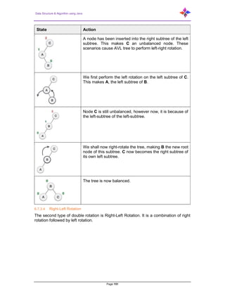


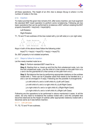
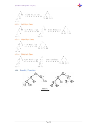

![Data Structure & Algorithm using Java
Page 157
6.8 B-Trees (or general m-way search trees)
Search tree called B-Tree in which a node can store more than one value (key) and it
can have more than two children. B-Tree was developed in the year 1972 by Bayer
and McCreight with the name Height Balanced m-way Search Tree. Later it was
named as B-Tree.
B-Tree can be defined as a self-balanced search tree with multiple keys in every node
and more than two children for every node.
Here, number of keys in a node and number of children for a node is depending on
the order of the B-Tree. Every B-Tree has order.
B-Tree of Order m has the following properties.
Property #1 - All the leaf nodes must be at same level.
Property #2 - All nodes except root must have at least [m/2]-1 keys and
maximum of m-1 keys.
Property #3 - All non-leaf nodes except root (i.e. all internal nodes) must have
at least m/2 children.
Property #4 - If the root node is a non-leaf node, then it must have at least 2
children.
Property #5 - A non-leaf node with n-1 keys must have n number of children.
Property #6 - All the key values within a node must be in Ascending Order.
For example, B-Tree of Order 4 contains maximum 3 key values in a node and
maximum 4 children for a node.
Example:](https://image.slidesharecdn.com/datastructurealgorithmusingjavav1-180530094707/85/Data-structure-algorithm-using-java-157-320.jpg)

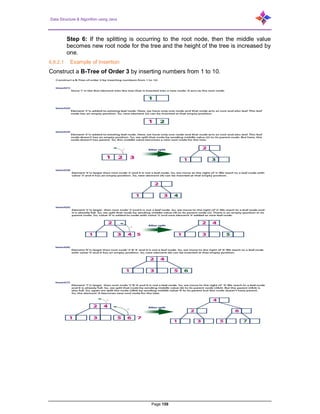
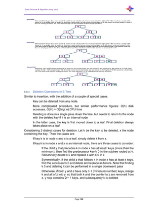


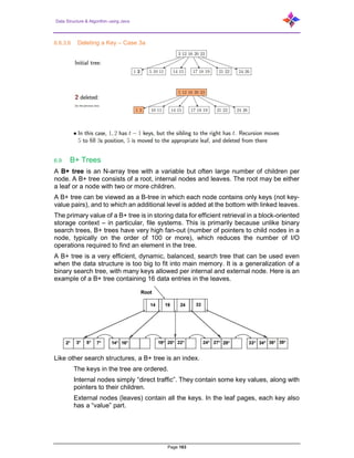
![Data Structure & Algorithm using Java
Page 164
So far, we have often considered pairs. With B+ trees, we can do this, too; however,
sometimes the “value” is a pointer (e.g. 10 bytes long) that contains the disk address
of the object to which the key applies (e.g., employee record/structure, video, file). This
is a great idea, especially when the data values would take up too many bytes of
memory/storage.
6.9.1 Order of a B+ tree
Let us define the order m of a B+ tree as the maximum number of data entries (e.g.
pairs) that can fit in a leaf page (node). Usually, longer keys (e.g. strings vs. integers)
mean that fewer data entries can fit in a leaf page. Note that different authors may
have different definitions of order. For example, some authors say that the order is:–
the minimum number d of search keys permitted by a non-root node. [Ramakrishnan
& Gehrke]. The maximum number of search keys that will fit in a node is therefore 2d,
which is what we call m– the maximum number d of children permitted in an internal
node [Silberschatz, Korth, & Sudarshan].
6.9.2 Properties of a B+ Tree of Order m
All leaves are on the same level. If a B+ tree consists of a single node, then the node
is both a root and a leaf. It’s an external node in this case, not an internal node. “Half-
full” rule,
part 1: Each leaf node (unless it’s a root) must contain between m/2 and m
pairs.
part 2: Each internal node other than the root has between (m+1)/2 and m+1
children, where m ≥ 2.
6.10 2-3 Trees
A 2–3 tree is a tree data structure where every node with children (internal node) has
either two children (2-node) and one data element or three children (3-nodes) and two
data elements. According to Knuth, “a B-tree of order 3 is a 2-3 tree.” Nodes on the
outside of the tree (leaf nodes) have no children and one or two data elements. 2−3
trees were invented by John Hopcroft in 1970.
2 nodes:
3 nodes:
2–3 trees are balanced, meaning that each right, center, and left subtree contains the
same or close to the same amount of data.
A 2-3 Tree is a specific form of a B tree. A 2-3 tree is a search tree. However, it is very
different from a binary search tree.](https://image.slidesharecdn.com/datastructurealgorithmusingjavav1-180530094707/85/Data-structure-algorithm-using-java-164-320.jpg)

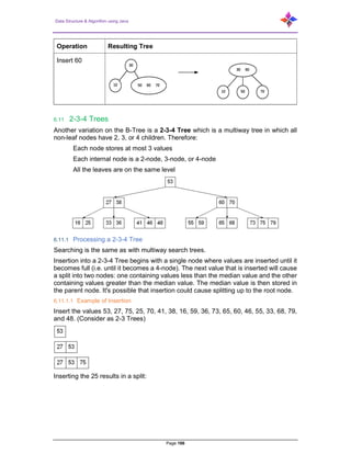

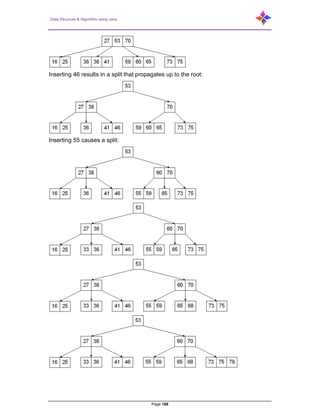
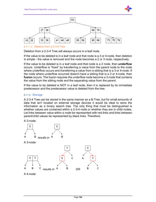

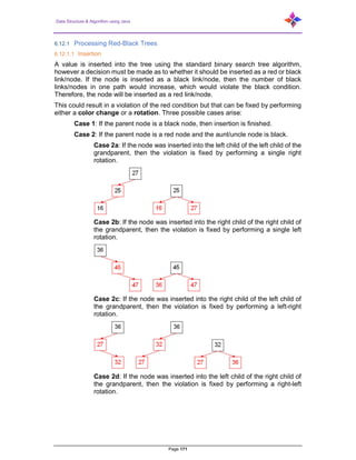


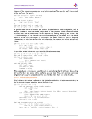


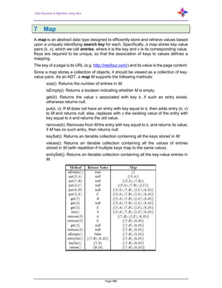
![Data Structure & Algorithm using Java
Page 184
7.1 Java Map Interface
A map contains values based on key i.e. key and value pair. Each key and value pair
is known as an entry. Map contains only unique keys.
Map is useful if you have to search, update, or delete elements based on key.
7.1.1 Useful methods of Map interface
Method Description
Object put(Object key, Object
value)
It is used to insert an entry in this map.
void putAll(Map map) It is used to insert the specified map in this map.
Object remove(Object key) It is used to delete an entry for the specified key.
Object get(Object key) It is used to return the value for the specified key.
boolean containsKey(Object
key)
It is used to search the specified key from this
map.
Set keySet() It is used to return the Set view containing all the
keys.
Set entrySet() It is used to return the Set view containing all the
keys and values.
Map implementation in JAVA:
package ADTList;
/**
* @author Narayan
*/
import java.util.*;
public class MapInterfaceExample {
public static void main(String args[] ) {
HashMap <Integer,String> map = new HashMap <Integer,String> ();
map.put(100,”Amit”);
map.put(101,”Vijay”);
map.put(102,”Rahul”);
map.put(101, “narayan”);
for(HashMap.Entry m:map.entrySet()) {
System.out.println(m.getKey()+” “+m.getValue());
}
}
}
7.2 Java LinkedHashMap class
Java LinkedHashMap class is Hash table and Linked list implementation of the Map
interface, with predictable iteration order. It inherits HashMap class and implements
the Map interface.](https://image.slidesharecdn.com/datastructurealgorithmusingjavav1-180530094707/85/Data-structure-algorithm-using-java-184-320.jpg)


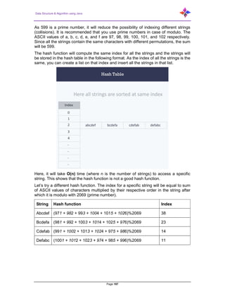


![Data Structure & Algorithm using Java
Page 190
7.3.3.2 Separate Chaining
A simple and efficient way for dealing with collisions is to have each bucket A[ j] store
its own secondary container, holding all entries (k, v) such that h(k) = j. A natural choice
for the secondary container is a small map instance implemented using an unordered
list.
7.4 The Set ADT
The Java Collections Framework defines the java.util.Set interface, which includes the
following fundamental methods:
add(e): Adds the element e to S (if not already present).
remove(e): Removes the element e from S (if it is present).](https://image.slidesharecdn.com/datastructurealgorithmusingjavav1-180530094707/85/Data-structure-algorithm-using-java-190-320.jpg)
![Data Structure & Algorithm using Java
Page 191
contains(e): Returns whether e is an element of S.
iterator(): Returns an iterator of the elements of S.
There is also support for the traditional mathematical set operations of union,
intersection, and subtraction of two sets S and T:
S ∪ T = {e: e is in S or e is in T},
S ∩ T = {e: e is in S and e is in T},
S − T = {e: e is in S and e is not in T}.
In the java.util.Set interface, these operations are provided through the following
methods, if executed on a set S:
addAll(T): Updates S to also include all elements of set T, effectively replacing
S by S ∪ T.
retainAll(T): Updates S so that it only keeps those elements that are also
elements of set T, effectively replacing S by S ∩ T.
removeAll(T): Updates S by removing any of its elements that also occur in set
T, effectively replacing S by S−T.
7.5 Linear Probing and Its Variants
A simple method for collision handling with open addressing is linear probing. With
this approach, if we try to insert an entry (k, v) into a bucket A[ j] that is already
occupied, where j = h(k), then we next try A[(j+1) mod N]. If A[(j+1) mod N] is also
occupied, then we try A[(j+2) mod N], and so on, until we find an empty bucket that
can accept the new entry. Once this bucket is located, we simply insert the entry there.
Of course, this collision resolution strategy requires that we change the
implementation when searching for an existing key—the first step of all get, put, or
remove operations. In particular, to attempt to locate an entry with key equal to k, we
must examine consecutive slots, starting from A[h(k)], until we either find an entry with
an equal key or we find an empty bucket.](https://image.slidesharecdn.com/datastructurealgorithmusingjavav1-180530094707/85/Data-structure-algorithm-using-java-191-320.jpg)


![Data Structure & Algorithm using Java
Page 194
Graphs are used to represent many real-life applications: Graphs are used to
represent networks. The networks may include paths in a city or telephone network or
circuit network. Graphs are also used in social networks like LinkedIn, Facebook. For
example, in Facebook, each person is represented with a vertex (or node). Each node
is a structure and contains information like person id, name, gender and locale.
Following is an example undirected graph with 5 vertices.
Following two are the most commonly used representations of graph.
Adjacency Matrix
Adjacency List
There are other representations also like, Incidence Matrix and Incidence List. The
choice of the graph representation is situation specific. It totally depends on the type
of operations to be performed and ease of use.
8.6 Graph Representation
8.6.1 Adjacency Matrix
Adjacency Matrix is a 2D array of size V x V where V is the number of vertices in a
graph. Let the 2D array be adj[][], a slot adj[i][j] = 1 indicates that there is an edge from
vertex i to vertex j. Adjacency matrix for undirected graph is always symmetric.
Adjacency Matrix is also used to represent weighted graphs. If adj[i][j] = w, then there
is an edge from vertex i to vertex j with weight w.
The adjacency matrix for the above example graph is:
Pros: Representation is easier to implement and follow. Removing an edge takes O(1)
time. Queries like vertex ‘u’ to vertex ‘v’ are connected by an edge are efficient and
can be done in O(1) time.
Cons: Consumes more space O(V^2). Even if the graph is sparse (contains less
number of edges), it consumes the same space. Adding a vertex takes O(V^2) time.
8.6.2 Adjacency List:
An array of linked lists is used. Size of the array is equal to number of vertices. Let the
array be array[]. An entry array[i] represents the linked list of vertices adjacent to the
ith vertex. This representation can also be used to represent a weighted graph. The](https://image.slidesharecdn.com/datastructurealgorithmusingjavav1-180530094707/85/Data-structure-algorithm-using-java-194-320.jpg)
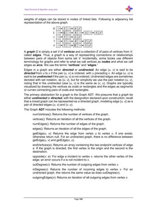
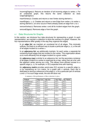
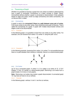
![Data Structure & Algorithm using Java
Page 198
By removing ‘e’ or ‘c’, the graph will become a disconnected graph.
Without ‘g’, there is no path between vertex ‘c’ and vertex ‘h’ and many other. Hence
it is a disconnected graph with cut vertex as ‘e’. Similarly, ‘c’ is also a cut vertex for the
above graph.
8.8.3 Cut Edge (Bridge)
Let ‘G’ be a connected graph. An edge ‘e’ ∈ G is called a cut edge if ‘G-e’ results in a
disconnected graph. If removing an edge in a graph results in to two or more graphs,
then that edge is called a Cut Edge.
8.8.3.1 Example
In the following graph, the cut edge is [(c, e)]
By removing the edge (c, e) from the graph, it becomes a disconnected graph.](https://image.slidesharecdn.com/datastructurealgorithmusingjavav1-180530094707/85/Data-structure-algorithm-using-java-198-320.jpg)


![Data Structure & Algorithm using Java
Page 202
because each vertex is connected with another vertex by an edge. Hence it has a
minimum degree of 1.
8.8.7.1 Example
Look at the following graph−
Its subgraphs having line covering are as follows−
C1 = {{a, b}, {c, d}}
C2 = {{a, d}, {b, c}}
C3 = {{a, b}, {b, c}, {b, d}}
C4 = {{a, b}, {b, c}, {c, d}}
Line covering of ‘G’ does not exist if and only if ‘G’ has an isolated vertex. Line covering
of a graph with ‘n’ vertices has at least [n – 2] edges.
8.8.8 Minimal Line Covering
A line covering C of a graph G is said to be minimal if no edge can be deleted from
C.
8.8.8.1 Example
In the above graph, the subgraphs having line covering are as follows−
C1 = {{a, b}, {c, d}}
C2 = {{a, d}, {b, c}}
C3 = {{a, b}, {b, c}, {b, d}}
C4 = {{a, b}, {b, c}, {c, d}}
Here, C1, C2, C3 are minimal line coverings, while C4 is not because we can delete
{b, c}.
8.8.9 Minimum Line Covering
It is also known as Smallest Minimal Line Covering. A minimal line covering with
minimum number of edges is called a minimum line covering of ‘G’. The number of
edges in a minimum line covering in ‘G’ is called the line covering number of ‘G’ (α1).
8.8.9.1 Example
In the above example, C1 and C2 are the minimum line covering of G and α1 = 2.
Every line covering contains a minimal line covering.
Every line covering does not contain a minimum line covering (C3 does not contain
any minimum line covering.
No minimal line covering contains a cycle.
If a line covering ‘C’ contains no paths of length 3 or more, then ‘C’ is a minimal line
covering because all the components of ‘C’ are star graph and from a star graph, no
edge can be deleted.](https://image.slidesharecdn.com/datastructurealgorithmusingjavav1-180530094707/85/Data-structure-algorithm-using-java-202-320.jpg)
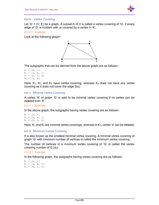

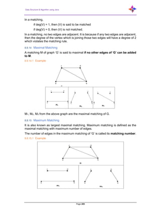


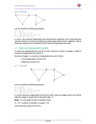

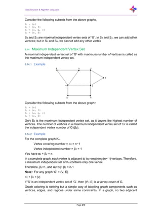
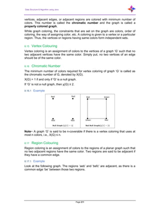

![Data Structure & Algorithm using Java
Page 213
Clustering
Data mining
Image capturing
Image segmentation
Networking
Resource allocation
Processes scheduling
A graph can exist in different forms having the same number of vertices, edges, and
the same edge connectivity. Such graphs are called isomorphic graphs. Note that we
label the graphs in this chapter mainly for referring to them and recognizing them from
one another.
8.19 Isomorphic Graphs
Two graphs G1 and G2 are said to be isomorphic if−
Their number of components (vertices and edges) are same.
Their edge connectivity is retained.
Note− In short, out of the two isomorphic graphs, one is a tweaked version of the
other. An unlabeled graph also can be thought of as an isomorphic graph.
There exists a function ‘f’ from vertices of G1 to vertices of G2
[f: V(G1) ⇒ V(G2)], such that
Case (i): f is a bijection (both one-one and onto)
Case (ii): f preserves adjacency of vertices, i.e., if the edge {U, V} ∈ G1, then
the edge {f(U), f(V)} ∈ G2, then G1 ≡ G2.
Note…
If G1 ≡ G2 then−
|V(G1)| = |V(G2)|
|E(G1)| = |E(G2)|
Degree sequences of G1 and G2 are same.
If the vertices {V1, V2, …, Vk} form a cycle of length K in G1, then the vertices {f(V1),
f(V2), …, f(Vk)} should form a cycle of length K in G2.
All the above conditions are necessary for the graphs G1 and G2 to be isomorphic, but
not sufficient to prove that the graphs are isomorphic.
(G1 ≡ G2) if and only if (G1− ≡ G2−) where G1 and G2 are simple graphs.
(G1 ≡ G2) if the adjacency matrices of G1 and G2 are same.
(G1 ≡ G2) if and only if the corresponding subgraphs of G1 and G2(obtained by
deleting some vertices in G1 and their images in graph G2) are isomorphic.](https://image.slidesharecdn.com/datastructurealgorithmusingjavav1-180530094707/85/Data-structure-algorithm-using-java-213-320.jpg)


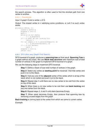


![Data Structure & Algorithm using Java
Page 226
void bfs(Graph g, int r) {
boolean[] seen = new boolean[g.nVertices()];
Queue<Integer> q = new SLList<Integer>();
q.add(r);
seen[r] = true;
while (!q.isEmpty()) {
int i = q.remove();
for (Integer j : g.outEdges(i)) {
if (!seen[j]) {
q.add(j);
seen[j] = true;
}
}
}
}
An example of running bfs(g, 0) on the graph is shown below. Different executions
are possible, depending on the ordering of the adjacency lists;
An example of bread-first-search starting at node 0. Nodes are labelled with the order
in which they are added to q. Edges that result in nodes being added to q are drawn
in black, other edges are drawn in grey.
Analyzing the running-time of the bfs(g, i) routine is straightforward. The use of the
seen array ensures that no vertex is added to q more than once. Adding (and later
removing) each vertex from q takes constant time per vertex for a total of O(n) time.
Since each vertex is processed by the inner loop at most once, each adjacency list is
processed at most once, so each edge of G is processed at most once. This
processing, which is done in the inner loop takes constant time per iteration, for a total
of O(m) time. Therefore, the entire algorithm runs in O(n+m) time.
The following theorem summarizes the performance of the bfs(g, r) algorithm.
When given as input a Graph, g, that is implemented using the AdjacencyLists data
structure, the bfs(g, r) algorithm runs in O(n+m) time.
A breadth-first traversal has some very special properties. Calling bfs(g, r) will
eventually enqueue (and eventually dequeue) every vertex j such that there is a
directed path from r to j. Moreover, the vertices at distance 0 from r (r itself) will enter
q before the vertices at distance 1, which will enter q before the vertices at distance
2, and so on. Thus, the bfs(g, r) method visits vertices in increasing order of distance
from r and vertices that cannot be reached from r are never visited at all.
A particularly useful application of the breadth-first-search algorithm is, therefore, in
computing shortest paths. To compute the shortest path from r to every other vertex,
we use a variant of bfs(g, r) that uses an auxiliary array, p, of length n. When a new
vertex j is added to q, we set p[j]=i. In this way, p[j] becomes the second last node](https://image.slidesharecdn.com/datastructurealgorithmusingjavav1-180530094707/85/Data-structure-algorithm-using-java-226-320.jpg)
![Data Structure & Algorithm using Java
Page 227
on a shortest path from r to j. Repeating this, by taking p[p[j], p[p[p[j]]], and so on we
can reconstruct the (reversal of) a shortest path from r to j.
The depth-first-search algorithm is similar to the standard algorithm for traversing
binary trees; it first fully explores one subtree before returning to the current node and
then exploring the other subtree. Another way to think of depth-first-search is by saying
that it is similar to breadth-first search except that it uses a stack instead of a queue.
During the execution of the depth-first-search algorithm, each vertex, i, is assigned a
colour, c[i]:white if we have never seen the vertex before, grey if we are currently
visiting that vertex, and black if we are done visiting that vertex. The easiest way to
think of depth-first-search is as a recursive algorithm. It starts by visiting r. When
visiting a vertex i, we first mark i as grey. Next, we scan i's adjacency list and
recursively visit any white vertex we find in this list. Finally, we are done processing i,
so we colour i black and return.
void dfs(Graph g, int r) {
byte[] c = new byte[g.nVertices()];
dfs(g, r, c);
}
void dfs(Graph g, int i, byte[] c) {
c[i] = grey; // currently visiting i
for (Integer j : g.outEdges(i)) {
if (c[j] == white) {
c[j] = grey;
dfs(g, j, c);
}
}
c[i] = black; // done visiting i
}
An example of the execution of this algorithm is shown below
An example of depth-first-search starting at node 0. Nodes are labelled with the order
in which they are processed. Edges that result in a recursive call are drawn in black,
other edges are drawn in grey.
Although depth-first-search may best be thought of as a recursive algorithm, recursion
is not the best way to implement it. Indeed, the code given above will fail for many
large graphs by causing a stack overflow. An alternative implementation is to replace
the recursion stack with an explicit stack s. The following implementation does that:
void dfs2(Graph g, int r) {
byte[] c = new byte[g.nVertices()];
Stack<Integer> s = new Stack<Integer>();
s.push(r);](https://image.slidesharecdn.com/datastructurealgorithmusingjavav1-180530094707/85/Data-structure-algorithm-using-java-227-320.jpg)
![Data Structure & Algorithm using Java
Page 228
while (!s.isEmpty()) {
int i = s.pop();
if (c[i] == white) {
c[i] = grey;
for (int j : g.outEdges(i))
s.push(j);
}
}
}
8.30 Application of Graph
Since they are powerful abstractions, graphs can be very important in modelling data.
In fact, many problems can be reduced to known graph problems. Here we outline just
some of the many applications of graphs.
Few important real-life applications of graph data structures are:
Facebook: Each user is represented as a vertex and two people are friends
when there is an edge between two vertices. Similarly, friend suggestion also
uses graph theory concept.
Google Maps: Various locations are represented as vertices and the roads are
represented as edges and graph theory is used to find shortest path between
two nodes.
Recommendations on e-commerce websites: The “Recommendations for
you” section on various e-commerce websites uses graph theory to recommend
items of similar type to user’s choice.
Graph theory is also used to study molecules in chemistry and physics.
Some other practical uses are as following:
Social network graphs: To tweet or not to tweet. Graphs that represent who
knows whom, who communicates with whom, who influences whom or other
relationships in social structures. An example is the twitter graph of who follows
whom. These can be used to determine how information flows, how topics
become hot, how communities develop, or even who might be a good match
for who, or is that whom.
Transportation networks. In road networks vertices are intersections and
edges are the road segments between them, and for public transportation
networks vertices are stops and edges are the links between them. Such
networks are used by many map programs such as Google maps, Bing maps
and now Apple IOS 6 maps (well perhaps without the public transport) to find
the best routes between locations. They are also used for studying traffic
patterns, traffic light timings, and many aspects of transportation.
Utility graphs. The power grid, the internet, and the water network are all
examples of graphs where vertices represent connection points, and edges the
wires or pipes between them. Analyzing properties of these graphs is very
important in understanding the reliability of such utilities under failure or attack,
or in minimizing the costs to build infrastructure that matches required
demands.](https://image.slidesharecdn.com/datastructurealgorithmusingjavav1-180530094707/85/Data-structure-algorithm-using-java-228-320.jpg)


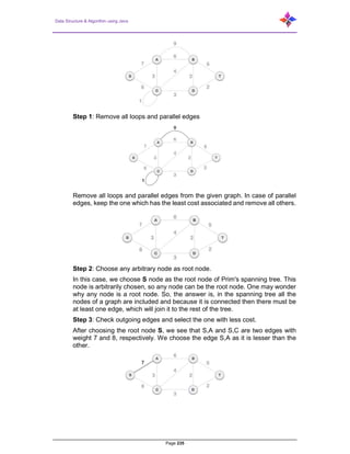
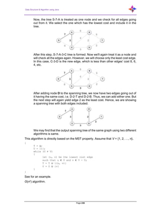
![Data Structure & Algorithm using Java
Page 237
9.7.1 Proof of Correctness of Prim's Algorithm
Theorem: Prim's algorithm finds a minimum spanning tree.
Proof: Let G = (V, E) be a weighted, connected graph. Let T be the edge set that is
grown in Prim's algorithm. The proof is by mathematical induction on the number of
edges in T and using the MST Lemma.
Basis: The empty set ф is promising since a connected, weighted graph always has
at least one MST.
Induction Step: Assume that T is promising just before the algorithm adds a new
edge e = (u, v). Let U be the set of nodes grown in Prim's algorithm. Then all three
conditions in the MST Lemma are satisfied and therefore T U e is also promising.
When the algorithm stops, U includes all vertices of the graph and hence T is a
spanning tree. Since T is also promising, it will be a MST.
9.7.2 Implementation of Prim's Algorithm
Use two arrays, closest and lowcost.
For i ∈ V - U, closest[i] gives the vertex in U that is closest to i
For i ∈ V - U, lowcost[i] gives the cost of the edge (i, closest(i))
Illustration of Prim's algorithm:
An example graph for illustrating Prim's algorithm:](https://image.slidesharecdn.com/datastructurealgorithmusingjavav1-180530094707/85/Data-structure-algorithm-using-java-237-320.jpg)
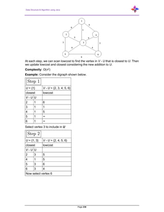


Data structure & algorithm using java
- 1. 2018 Data Structure & Algorithm using Java First Edition Narayan Sau P U N E , I N D I A
- 2. Data Structure & Algorithm using Java Page 2 Data Structure & Algorithm Using Java First Edition By Narayan Sau, MCA, MBA COPYRIGHT INFORMATION No part of this document may be copied, reproduced, stored in any retrieval system, or transmitted in any form or by any means, either electronically, mechanically, or otherwise without prior written permission. Neo Four Technologies LLP, April 2018 All rights reserved. Neo Four Technologies LLP, www.neofour.com
- 3. Data Structure & Algorithm using Java Page 3 Data Structure & Algorithm Using Java By Narayan Sau ॐ पूणमदः पूणिमदं पूणा ुणमुद ते पूण पूणमादाय पूणमेवाविश ते ॥ ॐ शा ः शा ः शा ः ॥ Om Puurnnam-Adah Puurnnam-Idam Puurnnaat-Purnnam-Udacyate Puurnnasya Puurnnam-Aadaaya Puurnnam-Eva-Avashissyate || Om Shaantih Shaantih Shaantih || Om, That is complete, This is complete, From the completeness comes the completeness If completeness is taken away from completeness, Only completeness remains Om, Peace peace peace To my wife Sonali, our children Adithya and Aditi
- 4. Data Structure & Algorithm using Java Page 4 Preface The great learning of my life is this: If you want to make a new contribution, you’ve got to make a new preparation. This book is written keeping this in mind. It will help students learn and understand data structure and algorithm and help them with their ides of developing product/app. This should also hold them in good stead in their attempt to get placed in a Software Product Company. We all know perfection does not leave any room for improvement. So, let’s keep the perfection aside, rather aim to concentrate ourselves and put our best attention in everything we do. Let us remember there is something you can do better than anyone else. Let’s not compare with or compete with others but with inner self. Let ask and get approval from inside rather looking for somebody’s nod. Let us find the one best thing in us and try to improve it in day by day. My intention behind writing this book is try to gather as much information as possible, which is freely available on internet, and summarize it all in knowledge form to help students scratch their head and concentrate in one place for understanding data structures. This book is made freely available for educational and other non-commercial use only. I am truly indebted to my reviewer Manish Chowdhury whose tireless efforts helped this book to see the dawn of the day by eradicating many technical errors, duplication, various spelling mistakes, and improved its readability. For any suggestion and comment please write to the author. (Narayan Sau)
- 5. Data Structure & Algorithm using Java Page 5 About the Author Narayan Sau. Over 23 years of experience in Telecom BSS domain. Expertise in BSS/OSS system integration, Test automation, Migration and DevOps. Founder and Director of Neo Four Technologies. MBA from University of Dallas, Texas, USA. LinkedIn: https://www.linkedin.com/in/narayansau/ Email: [email protected] About the Reviewer Manish Chowdhury. Over 20 years of extensive international IT Industry experience in Telecom domain, end-to-end IT services including complex IT Program and Project Management, Solution Design, Development, Testing, Delivery, and Operations Management, Leadership, and Team Building. MBA from University of Kansas, Kansas, USA LinkedIn: https://www.linkedin.com/in/manishc/ Email: [email protected]
- 6. Data Structure & Algorithm using Java Page 6 Table of Contents 1 Introduction to Algorithms and Data Structures.................................................. 17 1.1 Prerequisites....................................................................................................... 17 1.2 Role of Algorithm ................................................................................................ 17 1.2.1 Laymen terms........................................................................................................ 17 1.3 Role of a Data Structure...................................................................................... 18 1.4 Identifying Techniques for Designing Algorithms................................................. 19 1.4.1 Brute Force............................................................................................................ 19 1.4.2 Greedy Algorithms “take what you can get now” strategy .................................... 19 1.4.3 Divide-and-Conquer, Decrease-and-Conquer ...................................................... 21 1.4.4 Dynamic Programming.......................................................................................... 22 1.4.5 Transform-and-Conquer........................................................................................ 22 1.4.6 Backtracking and branch-and-bound: Generate and test methods ...................... 22 1.5 What is Data Structure........................................................................................ 23 1.5.1 Types of Data Structures....................................................................................... 23 1.5.2 Dynamic Memory Allocation.................................................................................. 24 1.6 Algorithm Analysis............................................................................................... 25 1.6.1 Big Oh Notation, Ο ................................................................................................ 26 1.6.2 Omega Notation, Ω................................................................................................ 26 1.6.3 Theta Notation, θ................................................................................................... 27 1.6.4 How to analyze a program .................................................................................... 27 1.6.4.1 Some Mathematical Facts ..................................................................... 31 1.7 Random Access Machine model......................................................................... 32 1.8 Abstract Data Type ............................................................................................. 33 1.8.1 Advantages of Abstract Data Typing..................................................................... 33 1.8.1.1 Encapsulation ........................................................................................ 33 1.8.1.2 Localization of change ........................................................................... 33 1.8.1.3 Flexibility ................................................................................................ 34 1.9 Arrays & Structure............................................................................................... 34 1.9.1 Types of an Array.................................................................................................. 34 1.9.1.1 One-dimensional array........................................................................... 34 1.9.1.2 Multi-dimensional array.......................................................................... 34 1.9.2 Array Declaration................................................................................................... 35 1.9.3 Array Initialization.................................................................................................. 35 1.9.4 Memory allocation ................................................................................................. 35 1.9.5 Advantages & Disadvantages ............................................................................... 35 1.9.5.1 Advantages ............................................................................................ 35 1.9.5.2 Disadvantages ....................................................................................... 36
- 7. Data Structure & Algorithm using Java Page 7 1.9.6 Bound Checking .................................................................................................... 36 2 Introduction to Stack, Operations on Stack ........................................................ 37 2.1 Stack Representation.......................................................................................... 37 2.2 Basic Operations................................................................................................. 38 2.2.1 peek() .................................................................................................................... 38 2.2.2 isfull()..................................................................................................................... 38 2.2.3 isempty()................................................................................................................ 38 2.2.4 Push Operation ..................................................................................................... 38 2.2.4.1 Algorithm for Push Operation ................................................................ 39 2.2.5 Pop Operation ....................................................................................................... 39 2.2.5.1 Algorithm for Pop Operation .................................................................. 40 2.2.6 Program on stack link implementation .................................................................. 40 2.2.7 My Stack Array Implementation ............................................................................ 42 2.2.8 Evaluation of Expression....................................................................................... 44 2.2.9 Infix, Prefix, Postfix................................................................................................ 45 2.2.10 Converting Between These Notations................................................................... 46 2.2.11 Infix to Postfix using Stack .................................................................................... 47 2.2.12 Evaluation of Postfix.............................................................................................. 48 2.2.13 Infix to Prefix using STACK................................................................................... 50 2.2.14 Evaluation of Prefix ............................................................................................... 50 2.2.15 Prefix to Infix Conversion ...................................................................................... 51 2.2.16 Tower of Hanoi...................................................................................................... 53 3 Introduction to Queue, Operations on Queue..................................................... 55 3.1 Applications of Queue......................................................................................... 55 3.2 Array implementation Of Queue.......................................................................... 55 3.3 Queue Representation........................................................................................ 56 3.4 Basic Operations................................................................................................. 56 3.4.1 peek() .................................................................................................................... 56 3.4.2 isfull()..................................................................................................................... 57 3.4.3 isempty()................................................................................................................ 57 3.5 Enqueue Operation............................................................................................. 57 3.6 Dequeue Operation............................................................................................. 58 3.7 Queue using Linked List...................................................................................... 58 3.8 Operations .......................................................................................................... 59 3.8.1 enQueue(value)..................................................................................................... 59 3.8.2 deQueue() ............................................................................................................. 59 3.8.3 display()– Displaying the elements of Queue........................................................ 60 3.8.3.1 Abstract Data Type definition of Queue/Dequeue ................................. 60 3.8.3.2 Linked List implementation of Queue .................................................... 62
- 8. Data Structure & Algorithm using Java Page 8 3.9 Deque ................................................................................................................. 64 3.10 Input Restricted Double Ended Queue................................................................ 65 3.11 Output Restricted Double Ended Queue ............................................................. 65 3.12 Circular Queue.................................................................................................... 70 3.12.1 Implementation of Circular Queue ........................................................................ 71 3.12.2 enQueue(value) - Inserting value into the Circular Queue.................................... 71 3.12.3 deQueue()– Deleting a value from the Circular Queue......................................... 72 3.12.4 display()– Displays the elements of a Circular Queue .......................................... 72 3.13 Priority Queue..................................................................................................... 72 3.14 Applications of the Priority Queue ....................................................................... 74 3.14.1 PriorityQueueSort.................................................................................................. 74 3.14.1.1 Algorithm................................................................................................ 74 3.15 Adaptable Priority Queues .................................................................................. 77 3.16 Multiple Queues .................................................................................................. 77 3.16.1 Method 1: Divide the array in slots of size n/k....................................................... 77 3.16.2 Method 2: A space efficient implementation ......................................................... 78 3.17 Applications of Queue Data Structure ................................................................. 78 3.18 Applications of Stack........................................................................................... 78 3.19 Applications of Queue......................................................................................... 79 3.20 Compare the data structures: stack and queue solution...................................... 79 3.21 Comparison Chart............................................................................................... 79 4 Linked List .......................................................................................................... 81 4.1 Why Linked List?................................................................................................. 81 4.2 Singly Linked List ................................................................................................ 81 4.2.1 Insertion................................................................................................................. 82 4.2.1.1 Inserting at Beginning of the list............................................................. 82 4.2.1.2 Inserting at End of the list ...................................................................... 83 4.2.1.3 Inserting at Specific location in the list (After a Node) ........................... 83 4.2.2 Deletion ................................................................................................................. 83 4.2.2.1 Deleting from Beginning of the list......................................................... 83 4.2.2.2 Deleting from End of the list................................................................... 84 4.2.2.3 Deleting a Specific Node from the list.................................................... 84 4.3 Displaying a Single Linked List............................................................................ 85 4.3.1 Algorithm ............................................................................................................... 85 4.4 Circular Linked List.............................................................................................. 87 4.4.1 Insertion................................................................................................................. 88 4.4.1.1 Inserting at Beginning of the list............................................................. 88 4.4.1.2 Inserting at End of the list ...................................................................... 88
- 9. Data Structure & Algorithm using Java Page 9 4.4.1.3 Inserting At Specific location in the list (After a Node)........................... 89 4.4.2 Deletion ................................................................................................................. 89 4.4.2.1 Deleting from Beginning of the list......................................................... 89 4.4.2.2 Deleting from End of the list................................................................... 90 4.4.2.3 Deleting a Specific Node from the list.................................................... 90 4.4.3 Displaying a circular Linked List............................................................................ 91 4.5 Doubly Linked List............................................................................................... 91 4.5.1 Insertion................................................................................................................. 92 4.5.1.1 Inserting at Beginning of the list............................................................. 92 4.5.1.2 Inserting at End of the list ...................................................................... 92 4.5.1.3 Inserting at Specific location in the list (After a Node) ........................... 93 4.5.2 Deletion ................................................................................................................. 93 4.5.2.1 Deleting from Beginning of the list......................................................... 93 4.5.2.2 Deleting from End of the list................................................................... 94 4.5.2.3 Deleting a Specific Node from the list.................................................... 94 4.5.3 Displaying a Double Linked List ............................................................................ 95 4.6 ADT Linked List................................................................................................... 95 4.7 ADT Doubly Linked List....................................................................................... 97 4.8 Doubly Circular Linked List................................................................................ 102 4.9 Insertion in Circular Doubly Linked List ............................................................. 103 4.9.1 Insertion at the end of list or in an empty list....................................................... 103 4.9.2 Insertion at the beginning of list .......................................................................... 103 4.9.3 Insertion in between the nodes of the list............................................................ 103 4.10 Advantages & Disadvantages of Linked List...................................................... 104 4.10.1 Advantages of Linked List ................................................................................... 104 4.10.1.1 Dynamic Data Structure....................................................................... 104 4.10.1.2 Insertion and Deletion.......................................................................... 104 4.10.1.3 No Memory Wastage ........................................................................... 104 4.10.1.4 Implementation .................................................................................... 104 4.10.2 Disadvantages of Linked List .............................................................................. 104 4.10.2.1 Memory Usage..................................................................................... 104 4.10.2.2 Traversal .............................................................................................. 104 4.10.2.3 Reverse Traversing.............................................................................. 104 4.11 Operations on Linked list................................................................................... 104 4.11.1 Algorithm for Concatenation................................................................................ 105 4.11.2 Searching ............................................................................................................ 105 4.11.2.1 Iterative Solution .................................................................................. 105 4.11.2.2 Recursive Solution............................................................................... 105 4.11.3 Polynomials Using Linked Lists........................................................................... 105
- 10. Data Structure & Algorithm using Java Page 10 4.11.4 Representation of Polynomial ............................................................................. 106 4.11.4.1 Representation of Polynomials using Arrays....................................... 106 4.12 Exercise on Linked List ..................................................................................... 106 5 Sorting & Searching Techniques...................................................................... 111 5.1 What is Sorting.................................................................................................. 111 5.2 Methods of Sorting (Internal Sort, External Sort)............................................... 111 5.3 Sorting Algorithms............................................................................................. 111 5.3.1 Bubble Sort.......................................................................................................... 111 5.3.2 Selection sort....................................................................................................... 113 5.3.2.1 How Selection Sort Works? ................................................................. 114 5.3.3 Insertion sort........................................................................................................ 115 5.3.4 Merge sort ........................................................................................................... 117 5.3.4.1 How Merge Sort Works?...................................................................... 118 5.3.4.2 Algorithm.............................................................................................. 118 5.3.5 Quick Sort............................................................................................................ 120 5.3.5.1 Analysis of Quick Sort.......................................................................... 120 5.3.6 Heap Sort ............................................................................................................ 121 5.3.6.1 What is Binary Heap? .......................................................................... 121 5.3.6.2 Why array based representation for Binary Heap? ............................. 121 5.3.6.3 Heap Sort algorithm for sorting in increasing order ............................. 121 5.3.6.4 How to build the heap? ........................................................................ 122 5.3.7 Radix Sort............................................................................................................ 123 5.4 Searching Techniques ...................................................................................... 124 5.4.1 Linear Search...................................................................................................... 124 5.4.2 Binary Search...................................................................................................... 125 5.4.3 Jump Search ....................................................................................................... 125 5.4.3.1 What is the optimal block size to be skipped?..................................... 125 5.4.4 Interpolation Search ............................................................................................ 125 5.4.4.1 Algorithm.............................................................................................. 126 5.4.5 Exponential Search ............................................................................................. 126 5.4.5.1 Applications of Exponential Search: .................................................... 126 5.4.6 Sublist Search (search a linked list in another list) ............................................. 126 5.4.7 Fibonacci Search................................................................................................. 127 5.4.7.1 Background.......................................................................................... 127 5.4.7.2 Observations........................................................................................ 128 5.4.7.3 Algorithm.............................................................................................. 128 5.4.7.4 Time Complexity Analysis.................................................................... 128 6 Trees................................................................................................................ 129 6.1 Definition of Tree............................................................................................... 129
- 11. Data Structure & Algorithm using Java Page 11 6.2 Tree Terminology.............................................................................................. 129 6.3 Terminology ...................................................................................................... 131 6.3.1 Root..................................................................................................................... 131 6.3.2 Edge .................................................................................................................... 132 6.3.3 Parent.................................................................................................................. 132 6.3.4 Child .................................................................................................................... 132 6.3.5 Siblings................................................................................................................ 133 6.3.6 Leaf...................................................................................................................... 133 6.3.7 Internal Nodes ..................................................................................................... 133 6.3.8 Degree................................................................................................................. 134 6.3.9 Level.................................................................................................................... 134 6.3.10 Height .................................................................................................................. 134 6.3.11 Depth................................................................................................................... 135 6.3.12 Path ..................................................................................................................... 135 6.3.13 Sub Tree.............................................................................................................. 135 6.4 Types of Tree.................................................................................................... 136 6.4.1 Binary Trees ........................................................................................................ 136 6.4.2 Binary Tree implementation in Java.................................................................... 137 6.5 Binary Search Trees ......................................................................................... 141 6.5.1 Adding a value..................................................................................................... 141 6.5.1.1 Search for a place................................................................................ 141 6.5.1.2 Insert a new element to this place ....................................................... 142 6.5.2 Deletion ............................................................................................................... 143 6.6 Heaps and Priority Queues ............................................................................... 144 6.6.1 Heaps .................................................................................................................. 144 6.6.1.1 Heap Implementation........................................................................... 145 6.6.2 Priority Queue ..................................................................................................... 147 6.6.2.1 Performance of Adaptable Priority Queue Implementations ............... 148 6.7 AVL Trees......................................................................................................... 148 6.7.1 Definition of an AVL tree ..................................................................................... 148 6.7.2 Insertion............................................................................................................... 149 6.7.3 AVL Rotations ..................................................................................................... 149 6.7.3.1 Left Rotation......................................................................................... 150 6.7.3.2 Right Rotation ...................................................................................... 150 6.7.3.3 Left-Right Rotation............................................................................... 150 6.7.3.4 Right-Left Rotation............................................................................... 151 6.7.4 AVL Tree | Set 1 (Insertion)................................................................................. 153 6.7.5 Why AVL Trees? ................................................................................................. 153 6.7.6 Insertion............................................................................................................... 154
- 12. Data Structure & Algorithm using Java Page 12 6.7.7 Steps to follow for insertion ................................................................................. 154 6.7.7.1 Left Left Case....................................................................................... 154 6.7.7.2 Left Right Case .................................................................................... 155 6.7.7.3 Right Right Case.................................................................................. 155 6.7.7.4 Right Left Case .................................................................................... 155 6.7.8 Insertion Examples.............................................................................................. 155 6.8 B-Trees (or general m-way search trees).......................................................... 157 6.8.1 Operations on a B-Tree....................................................................................... 158 6.8.1.1 Search Operation in B-Tree................................................................. 158 6.8.2 Insertion Operation in B-Tree.............................................................................. 158 6.8.2.1 Example of Insertion ............................................................................ 159 6.8.3 Deletion Operations in B Tree............................................................................. 160 6.8.3.1 Deleting a Key – Case 1 ...................................................................... 161 6.8.3.2 Deleting a Key – Cases 2a, 2b ............................................................ 161 6.8.3.3 Deleting a Key – Case 2c .................................................................... 162 6.8.3.4 Deleting a Key – Case 3b-1................................................................. 162 6.8.3.5 Deleting a Key – Case 3b-2................................................................. 162 6.8.3.6 Deleting a Key – Case 3a .................................................................... 163 6.9 B+ Trees ........................................................................................................... 163 6.9.1 Order of a B+ tree................................................................................................ 164 6.9.2 Properties of a B+ Tree of Order m..................................................................... 164 6.10 2-3 Trees .......................................................................................................... 164 6.10.1 Insertion............................................................................................................... 165 6.11 2-3-4 Trees ....................................................................................................... 166 6.11.1 Processing a 2-3-4 Tree...................................................................................... 166 6.11.1.1 Example of Insertion ............................................................................ 166 6.11.1.2 Deletion from a 2-3-4 Tree................................................................... 169 6.11.2 Storage................................................................................................................ 169 6.12 Red-Black Trees ............................................................................................... 170 6.12.1 Processing Red-Black Trees............................................................................... 171 6.12.1.1 Insertion ............................................................................................... 171 6.13 Applications of Binary Search Trees ................................................................. 172 6.13.1 Binary Search Tree ............................................................................................. 172 6.13.2 Binary Space Partition......................................................................................... 172 6.13.3 Binary Tries ......................................................................................................... 172 6.13.4 Hash Trees.......................................................................................................... 173 6.13.5 Heaps .................................................................................................................. 173 6.13.6 Huffman Coding Tree (Chip Uni)......................................................................... 173 6.13.7 GGM Trees.......................................................................................................... 173
- 13. Data Structure & Algorithm using Java Page 13 6.13.8 Syntax Tree ......................................................................................................... 173 6.13.9 Treap ................................................................................................................... 173 6.13.10 T-tree................................................................................................................... 173 6.14 Types of Binary Trees ....................................................................................... 173 6.14.1 Full Binary Tree ................................................................................................... 173 6.14.2 Complete Binary Tree ......................................................................................... 174 6.14.3 Perfect Binary Tree ............................................................................................. 174 6.14.4 Balanced Binary Tree.......................................................................................... 174 6.14.5 A degenerate (or pathological) tree..................................................................... 175 6.15 Representation of Binary Tree .......................................................................... 175 6.16 Array Implementation of Binary Tree................................................................. 176 6.17 Encoding Messages Using a Huffman Tree ...................................................... 176 6.17.1 Generating Huffman Trees.................................................................................. 178 6.17.2 Representing Huffman Trees .............................................................................. 179 6.17.2.1 The decoding procedure...................................................................... 180 6.17.2.2 Exercises ............................................................................................. 181 7 Map .................................................................................................................. 183 7.1 Java Map Interface............................................................................................ 184 7.1.1 Useful methods of Map interface ........................................................................ 184 7.2 Java LinkedHashMap class............................................................................... 184 7.3 Hash Table ....................................................................................................... 185 7.3.1 Hash function ...................................................................................................... 186 7.3.2 Need for a good hash function ............................................................................ 186 7.3.3 Collision resolution techniques............................................................................ 188 7.3.3.1 Separate chaining (open hashing)....................................................... 188 7.3.3.2 Separate Chaining ............................................................................... 190 7.4 The Set ADT ..................................................................................................... 190 7.5 Linear Probing and Its Variants ......................................................................... 191 8 Graphs ............................................................................................................. 192 8.1 What is a Graph? .............................................................................................. 192 8.2 Graph Terminology ........................................................................................... 192 8.3 Representation.................................................................................................. 192 8.3.1 Adjacency Matrix................................................................................................. 192 8.4 Adjacency List................................................................................................... 193 8.5 Graph and its representations ........................................................................... 193 8.6 Graph Representation....................................................................................... 194 8.6.1 Adjacency Matrix................................................................................................. 194 8.6.2 Adjacency List: .................................................................................................... 194
- 14. Data Structure & Algorithm using Java Page 14 8.7 Data Structures for Graphs ............................................................................... 196 8.8 Traversing a Graph ........................................................................................... 197 8.8.1 Connectivity......................................................................................................... 197 8.8.1.1 Example 1 ............................................................................................ 197 8.8.1.2 Example 2 ............................................................................................ 197 8.8.2 Cut Vertex ........................................................................................................... 197 8.8.2.1 Example ............................................................................................... 197 8.8.3 Cut Edge (Bridge)................................................................................................ 198 8.8.3.1 Example ............................................................................................... 198 8.8.4 Cut Set of a Graph .............................................................................................. 199 8.8.4.1 Example ............................................................................................... 199 8.8.5 Edge Connectivity ............................................................................................... 200 8.8.5.1 Example ............................................................................................... 200 8.8.6 Vertex Connectivity ............................................................................................. 200 8.8.6.1 Example 1 ............................................................................................ 200 8.8.6.2 Example 2 ............................................................................................ 201 8.8.7 Line Covering ...................................................................................................... 201 8.8.7.1 Example ............................................................................................... 202 8.8.8 Minimal Line Covering......................................................................................... 202 8.8.8.1 Example ............................................................................................... 202 8.8.9 Minimum Line Covering....................................................................................... 202 8.8.9.1 Example ............................................................................................... 202 8.8.10 Vertex Covering................................................................................................... 203 8.8.10.1 Example ............................................................................................... 203 8.8.11 Minimal Vertex Covering ..................................................................................... 203 8.8.11.1 Example ............................................................................................... 203 8.8.12 Minimum Vertex Covering................................................................................... 203 8.8.12.1 Example ............................................................................................... 203 8.8.13 Matching.............................................................................................................. 204 8.8.13.1 Example ............................................................................................... 204 8.8.14 Maximal Matching ............................................................................................... 205 8.8.14.1 Example ............................................................................................... 205 8.8.15 Maximum Matching ............................................................................................. 205 8.8.15.1 Example ............................................................................................... 205 8.8.16 Perfect Matching ................................................................................................. 206 8.8.16.1 Example ............................................................................................... 206 8.8.16.2 Example ............................................................................................... 206 8.8.16.3 Example ............................................................................................... 207 8.9 Independent Line Set........................................................................................ 207 8.9.1 Example............................................................................................................... 207
- 15. Data Structure & Algorithm using Java Page 15 8.10 Maximal Independent Line Set.......................................................................... 207 8.10.1 Example............................................................................................................... 208 8.11 Maximum Independent Line Set........................................................................ 208 8.11.1 Example............................................................................................................... 208 8.12 Independent Vertex Set .................................................................................... 209 8.12.1 Example............................................................................................................... 209 8.13 Maximal Independent Vertex Set ...................................................................... 209 8.13.1 Example............................................................................................................... 209 8.14 Maximum Independent Vertex Set .................................................................... 210 8.14.1 Example............................................................................................................... 210 8.14.2 Example............................................................................................................... 210 8.15 Vertex Colouring ............................................................................................... 211 8.16 Chromatic Number............................................................................................ 211 8.16.1 Example............................................................................................................... 211 8.17 Region Colouring .............................................................................................. 211 8.17.1 Example............................................................................................................... 211 8.18 Applications of Graph Colouring........................................................................ 212 8.19 Isomorphic Graphs............................................................................................ 213 8.19.1 Example............................................................................................................... 214 8.20 Planar Graphs................................................................................................... 214 8.20.1 Example............................................................................................................... 214 8.21 Regions............................................................................................................. 214 8.21.1 Example............................................................................................................... 215 8.22 Homomorphism................................................................................................. 216 8.23 Polyhedral graph............................................................................................... 217 8.24 Euler’s Path....................................................................................................... 218 8.25 Euler’s Circuit.................................................................................................... 218 8.26 Euler’s Circuit Theorem..................................................................................... 218 8.27 Hamiltonian Graph ............................................................................................ 219 8.28 Hamiltonian Path............................................................................................... 219 8.29 Graph traversal ................................................................................................. 220 8.29.1 Depth-first search ................................................................................................ 221 8.29.1.1 Pseudocode ......................................................................................... 221 8.29.2 Breadth-first search ............................................................................................. 221 8.29.2.1 Pseudocode ......................................................................................... 222 8.29.3 DFS other way (Depth First Search) ................................................................... 222 8.29.4 BFS other way (Breadth First Search) ................................................................ 224 8.30 Application of Graph.......................................................................................... 228
- 16. Data Structure & Algorithm using Java Page 16 8.31 Spanning Trees................................................................................................. 230 8.32 Circuit Rank ...................................................................................................... 230 8.33 Kirchoff’s Theorem............................................................................................ 231 9 Examples of Graph........................................................................................... 232 9.1 Example 1......................................................................................................... 232 9.1.1 Solution................................................................................................................ 232 9.2 Example 2......................................................................................................... 232 9.2.1 Solution................................................................................................................ 232 9.3 Example 3......................................................................................................... 233 9.3.1 Solution................................................................................................................ 233 9.4 Example 4......................................................................................................... 233 9.4.1 Solution................................................................................................................ 233 9.5 Example 5......................................................................................................... 233 9.5.1 Solution................................................................................................................ 233 9.6 Example 6......................................................................................................... 234 9.6.1 Solution................................................................................................................ 234 9.7 Prim’s Algorithm................................................................................................ 234 9.7.1 Proof of Correctness of Prim's Algorithm ............................................................ 237 9.7.2 Implementation of Prim's Algorithm..................................................................... 237 9.8 Kruskal’s Algorithm ........................................................................................... 239 9.8.1 Greedy algorithm................................................................................................. 239 9.8.2 Proof of Correctness of Kruskal's Algorithm ....................................................... 239 9.8.3 An illustration of Kruskal's algorithm ................................................................... 240 9.8.4 Program............................................................................................................... 241 9.8.5 Implementation.................................................................................................... 241 9.8.6 Running Time of Kruskal's Algorithm .................................................................. 241 9.8.7 Program............................................................................................................... 242 9.8.8 Implementation.................................................................................................... 243 9.8.9 Running Time of Kruskal's Algorithm .................................................................. 243 10 Complexity Theory ........................................................................................... 244 10.1 Undecidable Problems...................................................................................... 244 10.2 P Class Problems ............................................................................................. 244 10.3 NP Class Problems........................................................................................... 244 10.4 NP-Complete Problems .................................................................................... 245 10.5 NP-Hard............................................................................................................ 245
- 17. Data Structure & Algorithm using Java Page 17 1 Introduction to Algorithms and Data Structures 1.1 Prerequisites In presenting this book on data structure & algorithm, it is assumed that the reader has basic familiarity with any one of the high-level languages like Java, Python, C/C++. At the very least they are expected to know: Variables and Expressions Methods Conditional and loops Array, ADT 1.2 Role of Algorithm A program is a collection of instructions that performs a specific task when executed. A part of a computer program that performs a well-defined task is known as an algorithm. Let us concentrate on algorithms that are much underpins of today's computer programming. There are many steps involved in writing computer program to solve a given problem. The steps go from problem formulation and specification, to design of the solution, to implementation, testing and documentation, and finally to evaluation of the solution. The word algorithm comes from the name of the 9th century Persian and Muslim mathematician Abu Abdullah Muhammad ibn Musa Al-Khwarizmi. He was a mathematician, astronomer, and geographer during the Abbasid Caliphate, a scholar in the House of Wisdom in Baghdad. 1.2.1 Laymen terms An algorithm is a procedure to get things done. Precisely, An algorithm is a procedure to solve a problem in mathematical terms. It is the mathematical counterpart to programs. The essential concept to build efficient systems in space and time complexity and develop one’s problem solving skills. Provides the right set of techniques for data handling Helps you compare the efficiency of different approaches to a problem An important part of every technical interview round Given an algorithm, it can be implemented in any programming language. Similarly, all programs have an underlying algorithm which dictates their working. An algorithm as defined by Knuth must have the following properties: Finiteness. An algorithm must always terminate after a finite number of steps.
- 18. Data Structure & Algorithm using Java Page 18 Definiteness. Each step of an algorithm must be precisely defined down to the last detail. The action to be carried out must be rigorously and unambiguously specified for each case. Input. An algorithm has zero or more inputs. Output. An algorithm has one or more outputs. Effectiveness. An algorithm is also generally expected to be effective in the sense that its operations must all be sufficiently basic that they can in principle be done exactly and in a finite length of time by someone using pencil and paper. Let us explain with an example. Consider the simplest problem of finding the G.C.D. (H.C.F.) of two positive integer number m and n where n < m. E1. [Find remainder.] Divide m by n and let r be the remainder. ( 0<=r<n) E2. [Is it zero?] If r = 0, the algorithm terminates; n is the answer. E3. [Reduce] Set m =n, n = r. go back to step E1. The algorithm is terminating after finite number of steps [Finiteness]. All three steps are precisely defined [Definiteness]. The actions carrying out are rigorous and unambiguous. It has two [Input] and one [Output]. Also, the algorithm is effective in the sense that its operations can be done in finite length of time [Effectiveness]. 1.3 Role of a Data Structure A problem can be solved with multiple algorithms. Therefore, we need to choose an algorithm which provides maximum efficiency i.e. use minimum time and minimum memory. Thus, data structures come into picture. Data structure is the art of structuring the data in computer memory in such a way that the resulting operations can be performed efficiently. Data can be organized in many ways; therefore, you can create as many data structures as you want. However, there are some standard data structures that have proved to be useful over the years. These include arrays, linked lists, stacks, queues, trees, and graphs. We will learn more about these data structures in the subsequent sections. All these data structures are designed to hold a collection of data items. However, the difference lies in the way the data items are arranged with respect to each other and the operations that they allow. Because of the different ways in which the data items are arranged with respect to each other, some data structures prove to be more efficient than others in solving a given problem.
- 19. Data Structure & Algorithm using Java Page 19 1.4 Identifying Techniques for Designing Algorithms To solve our real-world problems, we need real world solutions. That’s why we may not follow any systematic method for designing an algorithm. But still there are some well-known techniques that have proved to be quite useful in designing algorithms. We follow these methods because: They provide templates suited to solving a broad range of diverse problems. They can be translated into common control and data structures provided by most high-level languages. The temporal and spatial requirements of the algorithms which result can be precisely analyzed. Although more than one technique may be applicable to a specific problem, it is often the case that an algorithm constructed by one approach is clearly superior to equivalent solutions built using alternative techniques. 1.4.1 Brute Force Brute force is a straightforward approach to solve a problem based on the problem statement and definitions of the concepts involved. It is considered as one of the easiest approach to apply and is useful for solving small-size instances of a problem. Some examples of brute force algorithms are: Computing an (a > 0, n a nonnegative integer) by multiplying a*a*…*a Computing n! Selection sort Bubble sort Sequential search Exhaustive search: Travelling Salesman Problem, Knapsack problem. 1.4.2 Greedy Algorithms “take what you can get now” strategy The greedy approach is an algorithm design technique that selects the best possible option at any given time. Algorithms based on the greedy approach are used for solving optimization problems, where you need to maximize profits or minimize costs under a given set of conditions. Some examples of optimization problems are: Finding the shortest distance from an originating city to a set of destination cities, given the distances between the pairs of cities. Finding the minimum number of currency notes required for an amount, where an arbitrary number of notes for each denomination are available. Selecting items with maximum value from a given set of items, where the total weight of the selected items cannot exceed a given value. Consider an example where you must fill a bag of 10 kg capacity by selecting items (from a set of items), whose weights and values are given in the following table:
- 20. Data Structure & Algorithm using Java Page 20 Item Weight (in kg) Value (in $/kg) Total Value (in $) A 2 200 400 B 3 150 450 C 4 200 800 D 1 50 50 E 5 100 500 A greedy algorithm acts greedy, and therefore selects the item with the maximum total value at each stage. Therefore, first item C with total value of $800 and weight 4 kgs will be selected. Next, item E with total value $500 and weight 5 kg will be selected. The next item with the highest value is item B with a total value of $450 and weight 3 kgs. However, if this item is selected, the total weight of the selected items will be 12 kgs (4 + 5 + 3), which is more than the capacity of the bag. Therefore, we discard item B and search for the item with the next highest value. The item with the next higher value is item A having a total value of $400 and a total weight of 2 kgs. However, the item also cannot be selected because if it is selected, the total weight of the selected items will be 11 kgs (4 + 5 + 2). Now, there is only one item left, that is, item D with a total value of $50 and a weight of 1 kg. This item can be selected as it makes the total weight equal to 10 kgs. The selected items and their total weights are listed in the following table: Item Weight (in kg) Total value (in $) C 4 800 E 5 500 D 1 50 Total 10 1350 Items selected using Greedy Approach: For most problems, greedy algorithms usually fail to find the globally optimal solution. This is because they usually don’t operate exhaustively on all data. They can make commitments to certain choices too early, which prevent them from finding the best overall solution later. This can be seen from the preceding example where the use of a greedy algorithm selects item with a total value of $1350 only. However, if the items were selected in the sequence depicted by the following table, the total value would have been much greater, with the weight being 10 kg only.
- 21. Data Structure & Algorithm using Java Page 21 Item Weight (in kg) Total value (in $) C 4 800 B 3 450 A 2 400 D 1 50 Total 10 1700 Optimal selection of Items: In the preceding example you can observe that the greedy approach commits to item E very early. This prevents it from determining the best overall solution later. Nevertheless, greedy approach is useful because it’s quick and easy to implement. Moreover, it often gives good approximation to the optimal value. 1.4.3 Divide-and-Conquer, Decrease-and-Conquer Given an instance of the problem to be solved, split this into several smaller sub- instances (of the same problem), independently solve each of the sub-instances, and then combine the sub-instance solutions to yield a solution for the original instance. With the divide-and-conquer method the size of the problem instance is reduced by a factor (e.g. half the input size), while with the decrease-and-conquer method the size is reduced by a constant. When we use recursion, the solution of the minimal instance is called “terminating condition”. Examples: Divide and Conquer Computing an (a > 0, n a nonnegative integer) by recursion Binary search in a sorted array (recursion) Merge sort algorithm, Quick sort algorithm (recursion) The algorithm for solving the fake coin problem (recursion) Decrease-and-Conquer Insertion sort Topological sorting Binary Tree traversals: inorder, preorder and postorder (recursion) Computing the length of the longest path in a binary tree (recursion) Computing Fibonacci numbers (recursion) Reversing a queue (recursion)
- 22. Data Structure & Algorithm using Java Page 22 1.4.4 Dynamic Programming One disadvantage of using Divide-and-Conquer is that the process of recursively solving separate sub-instances can result in the same computations being performed repeatedly since identical sub-instances may arise. The idea behind dynamic programming is to avoid this pathology by obviating the requirement to calculate the same quantity twice. The method usually accomplishes this by maintaining a table of sub-instance results. Dynamic Programming is a Bottom-Up technique in which the smallest sub-instances are explicitly solved first and the results of these are used to construct solutions to progressively larger sub-instances. In contrast, Divide-and-Conquer is a Top-Down technique which logically progresses from the initial instance down to the smallest sub-instance via intermediate sub- instances. 1.4.5 Transform-and-Conquer These methods work as two-stage procedures. First, the problem is modified to be more amenable to solution. In the second stage the problem is solved. Many problems involving lists are easier when list is sorted. Searching Computing the median (selection problem) Checking if all elements are distinct (element uniqueness) Pre-sorting is used in many geometric algorithms. Efficiency of algorithms involving sorting depends on efficiency of sorting. 1.4.6 Backtracking and branch-and-bound: Generate and test methods The method is used for state-space search problems. State-space search problems are problems, where the problem representation consists of: Initial state Goal state(s) A set of intermediate states A set of operators that transform one state into another. Each operator has pre- conditions and post-conditions. A cost function; evaluates the cost of the operations (optional) A utility function; evaluates how close is a given state to the goal state (optional) Example: You are given two jugs, a 4 gallon one and a 3 gallon one. Neither have any measuring markers on it. There is a tap that can be used to fill the jugs with water. How can you get exactly 2 gallons of water into the 4-gallon jug? Description Pre-conditions on (X, Y) Action (Post-conditions)
- 23. Data Structure & Algorithm using Java Page 23 O1. Fill A X < 4 (4, Y) O2. Fill B Y < 3 (X, 3) O3. Empty A X > 0 (0, Y) O4. Empty B Y > 0 (X, 0) O5. Pour A into B X > 3 - Y X ≤ 3 - Y (X + Y - 3, 3) (0, X + Y) O6. Pour B into A Y > 4 - X Y ≤ 4 - X (4, X + Y - 4) (X + Y, 0) 1.5 What is Data Structure A data structure is a specialized format for organizing and storing data. General data structure types include the array, the file, the record, the table, the tree, and so on. Any data structure is designed to organize data to suit a specific purpose so that it can be accessed and worked within appropriate ways. In computer programming, a data structure may be selected or designed to store data for working on it with various algorithms. 1.5.1 Types of Data Structures Following are the various types of data structures. Primitive types: Boolean, true or false. Character Floating-point, single-precision real number values. Double, a wider floating-point size. Integer, integral or fixed-precision values. String, a sequence of characters. Reference (also called a pointer or handle), a small value referring to another object's address in memory, possibly a much larger one. Enumerated type, a small set of uniquely named values. Composite types or Non-primitive type: Array Record (also called tuple or structure) Union Tagged unions (also called variant, variant record, discriminated union, or disjoint union)
- 24. Data Structure & Algorithm using Java Page 24 Abstract data types: Container List Associative array Multicar Set Multistep (Bag) Stack Queue Double-ended queue Priority queue Tree Graph Linear data structures: Arrays Types of Lists Trees Binary trees B-trees Heaps Trees Multiday trees Space-partitioning trees Application-specific trees Hashes Graphs 1.5.2 Dynamic Memory Allocation Dynamic memory allocation is when an executing program requests that the operating system give it a block of main memory. The program then uses this memory for some purpose. Usually the purpose is to add a node to a data structure. In object oriented languages, dynamic memory allocation is used to get the memory for a new object. The memory comes from above the static part of the data segment. Programs may request memory and may also return previously dynamically allocated memory. Memory may be returned whenever it is no longer needed. Memory can be returned in any order without any relation to the order in which it was allocated. The heap may develop “holes” where previously allocated memory has been returned between blocks of memory still in use.
- 25. Data Structure & Algorithm using Java Page 25 A new dynamic request for memory might return a range of addresses out of one of the holes. But it might not use up the entire hole, so further dynamic requests might be satisfied out of the original hole. If too many small holes develop, memory is wasted because the total memory used by the holes may be large, but the holes cannot be used to satisfy dynamic requests. This situation is called memory fragmentation. Keeping track of allocated and de- allocated memory is complicated. A modern operating system does all this. Memory for an object can also be allocated dynamically during a method's execution, by having that method utilize the special new operator built into Java. For example, the following Java statement creates an array of integers whose size is given by the value of variable k: int[] items = new int[k]; The size of the array above is known only at runtime. Moreover, the array may continue to exist even after the method that created it terminates. Thus, the memory for this array cannot be allocated on the Java stack. 1.6 Algorithm Analysis The analysis of algorithms is the determination of the computational complexity of algorithms, i.e. the amount of time, storage and/or other resources necessary to execute them. Usually, this involves determining a function that relates the length of an algorithm's input to the number of steps it takes (its time complexity) or the number of storage locations it uses (its space complexity). An algorithm is said to be efficient when this function's values are small. Since different inputs of the same length may cause the algorithm to have different behavior, the function describing its performance is usually an upper bound on the actual performance, determined from the worst case inputs to the algorithm. A Priori Analysis− This is a theoretical analysis of an algorithm. Efficiency of an algorithm is measured by assuming that all other factors, for example, processor speed, are constant and have no effect on the implementation. A Posterior Analysis− This is an empirical analysis of an algorithm. The selected algorithm is implemented using programming language. This is then executed on target computer machine. In this analysis, actual statistics like running time and space required, are collected. Time Factor− Time is measured by counting the number of key operations such as comparisons in the sorting algorithm. Space Factor− Space is measured by counting the maximum memory space required by the algorithm. In general, the running time of an algorithm or data structure method increases with the input size, although it may also vary for different inputs of the same size. Also, the running time is affected by the hardware environment (as reflected in the processor, clock rate, memory, disk, etc.) and software environment (as reflected in the operating system, programming language, compiler, interpreter, etc.) in which the algorithm is implemented, compiled, and executed. All other factors being equal, the running time of the same algorithm on the same input data will be smaller if the computer has, say, a much faster processor or if the implementation is done in a program compiled into
- 26. Data Structure & Algorithm using Java Page 26 native machine code instead of an interpreted implementation run on a virtual machine. Nevertheless, despite the possible variations that come from different environmental factors, we would like to focus on the relationship between the running time of an algorithm and the size of its input. We are interested in characterizing an algorithm's running time as a function of the input size. But what is the proper way of measuring it? Usually, the time required by an algorithm falls under three types: Best Case− Minimum time required for program execution. Average Case− Average time required for program execution. Worst Case− Maximum time required for program execution. Following are the commonly used asymptotic notations to calculate the running time complexity of an algorithm. Ο Notation Ω Notation θ Notation 1.6.1 Big Oh Notation, Ο The notation Ο(n) is the formal way to express the upper bound of an algorithm's running time. It measures the worst-case time complexity or the longest amount of time an algorithm can possibly take to complete. Let f(n) and g(n) be functions mapping non-negative integers to real numbers. We say that f(n) is O(g(n)) if there is a real constant c > 0 and an integer constant n0 >= 1 such that f(n) <= c.g(n), for n > n0. Then f(n) is big-Oh of g(n). 1.6.2 Omega Notation, Ω The notation Ω(n) is the formal way to express the lower bound of an algorithm's running time. It measures the best-case time complexity or the best amount of time an algorithm can possibly take to complete.
- 27. Data Structure & Algorithm using Java Page 27 If f(n) >= c.g(n) for c = constant and n > n0, then we say that f(n) is Ω(g(n)) 1.6.3 Theta Notation, θ Theta, commonly written as Θ, is an Asymptotic Notation to denote the asymptotically tight bound on the growth rate of runtime of an algorithm. f(n) is Θ(g(n)), if for some real constants c1, c2 and n0 (c1 > 0, c2 > 0, n0 > 0), c1 g(n) is < f(n) is < c2 g(n) for every input size n (n > n0). ∴ f(n) is Θ(g(n)) implies f(n) is O(g(n)) as well as f(n) is Ω(g(n)). The notation θ(n) is the formal way to express both the lower bound and the upper bound of an algorithm's running time. It is represented as follows− Notation name: O(1) constant O(log(n)) logarithmic O((log(n))^c) poly logarithmic O(n) linear O(n^2) quadratic O(n^c) polynomial O(c^n) exponential 1.6.4 How to analyze a program In general, how can you determine running time of a piece of code? The answer is that it depends on what kinds of statements are used. Let the sequence of statements be: statement 1; statement 2; … statement k; The total time is found by adding the times for all statements: total time = time(statement 1) + time(statement 2) + … + time(statement k) If each statement is “simple” (only involves basic operations) then the time for each statement is constant and the total time is also constant: O(1).
- 28. Data Structure & Algorithm using Java Page 28 If-Then-Else: if (condition) then block 1 (sequence of statements) else block 2 (sequence of statements) end if; Here, either block 1 will execute, or block 2 will execute. Therefore, the worst-case time is the slower of the two possibilities: max(time(block 1), time(block 2)) If block 1 takes O(1) and block 2 takes O(N), the if-then-else statement would be O(N). Loops: for I in 1.. N loop sequence of statements end loop; The loop executes N times, so the sequence of statements also executes N times. If we assume the statements are O(1), the total time for the for loop is N * O(1), which is O(N) Example (nested loops): for I in 1.. N loop for J in 1 … M loop sequence of statements end loop; end loop; The outer loop executes N times. Every time the outer loop executes, the inner loop executes M times. As a result, the statements in the inner loop execute a total of N*M times. Thus, the complexity is O(N*M). In a common special case where the stopping condition of the inner loop is never occurred, meaning the inner loop also executes N times, then the total complexity for the two loops is O(N^2). Statements with function/procedure calls When a statement involves a function/procedure call, the complexity of the statement includes the complexity of the function/procedure. Assuming that you know that function/procedure f takes constant time, and that function/procedure g takes time proportional to (linear in) the value of its parameter k. Then the statements below have the time complexities indicated. f(k) has O(1) g(k) has O(k) When a loop is involved, the same rule applies. For example: for J in 1.. N loop g(J); end loop; has complexity (N^2). The loop executes N times and each function/procedure call is of complexity O(N).
- 29. Data Structure & Algorithm using Java Page 29 CENG 213 Data Structures 12 Algorithm Growth Rates (cont.) Time requirements as a function of the problem size n
- 30. Data Structure & Algorithm using Java Page 30
- 31. Data Structure & Algorithm using Java Page 31 1.6.4.1 Some Mathematical Facts
- 32. Data Structure & Algorithm using Java Page 32 CENG 213 Data Structures 28 Growth-Rate Functions – Example3 Cost Times for (i=1; i<=n; i++) c1 n+1 for (j=1; j<=i; j++) c2 for (k=1; k<=j; k++) c3 x=x+1; c4 T(n) = c1*(n+1) + c2*( ) + c3* ( ) + c4*( ) = a*n3 + b*n2 + c*n + d So, the growth-rate function for this algorithm is O(n3) n j j 1 )1( n j j k k 1 1 )1( n j j k k 1 1 n j j 1 )1( n j j k k 1 1 )1( n j j k k 1 1 CENG 213 Data Structures 38 How much better is O(log2n)? n O(log2n) 16 4 64 6 256 8 1024 (1KB) 10 16,384 14 131,072 17 262,144 18 524,288 19 1,048,576 (1MB) 20 1,073,741,824 (1GB) 30 1.7 Random Access Machine model Algorithms can be measured in a machine-independent way using the Random Access Machine (RAM) model. This model assumes a single processor. In the RAM model, instructions are executed one after the other, with no concurrent operations. This model of computation is an abstraction that allows us to compare algorithms based on performance. The assumptions made in the RAM model to accomplish this are: Each simple operation takes 1-time step.
- 33. Data Structure & Algorithm using Java Page 33 Loops and subroutines are not simple operations. Each memory access takes one-time step, and there is no shortage of memory. For any given problem the running time of an algorithm is assumed to be the number of time steps. The space used by an algorithm is assumed to be the number of RAM memory cells. Elementary data-structures: arrays, lists, queues, stacks and their applications 1.8 Abstract Data Type The term ADT refers to Abstract Data Type in Data Structures. ADT is a conceptual model of information structure. An ADT specifies the components, their structuring relationships and a list of operations that can be performed. ADTs are independent of data representation and implementation of operations. It is just a specification; no design or implementation info is included. Specification involves the what’s of the operations, not the how’s. Suppose, in stack ADT you know what you want to do with that data structure. The methods i.e. push, pop, checking if the stack is empty or not, and the details of these methods are part of ADT. You can implement a stack using a 1-D array or linked list but we don't bother about these implementation details while defining ADT. Example: abstract stack (functional) For example, a complete functional-style definition of a stack ADT could use the three operations: push: takes a stack state and an arbitrary value, returns a stack state; top: takes a stack state, returns a value; pop: takes a stack state, returns a stack state; with the following axioms: top(push(s,x)) = x (pushing an item onto a stack leaves it at the top) pop(push(s,x)) = s (pop undoes the effect of push) 1.8.1 Advantages of Abstract Data Typing 1.8.1.1 Encapsulation Abstraction provides a promise that any implementation of the ADT has certain properties and abilities; knowing these is all that is required to make use of an ADT object. The user does not need any technical knowledge of how the implementation works to use the ADT. In this way, the implementation may be complex but will be encapsulated in a simple interface when it is used. 1.8.1.2 Localization of change Code that uses an ADT object will not need to be edited if the implementation of the ADT is changed. Since any changes to the implementation must still comply with the interface, and since code using an ADT may only refer to properties and abilities specified in the interface, changes may be made to the implementation without requiring any changes in code where the ADT is used.
- 34. Data Structure & Algorithm using Java Page 34 1.8.1.3 Flexibility Different implementations of an ADT, having all the same properties and abilities, are equivalent and may be used somewhat interchangeably in code that uses the ADT. This gives a great deal of flexibility when using ADT objects in different situations. For example, different implementations of an ADT may be more efficient in different situations; it is possible to use each in the situation where they are preferable, thus increasing overall efficiency. 1.9 Arrays & Structure Array is a fixed-size sequenced collection of variables belonging to the same data types. The array has adjacent memory locations to store values. An array data structure stores several elements of the same type in a specific order. They are accessed using an integer to specify which element is required (although the elements may be of almost any type). Arrays may be fixed-length or expandable. When data objects are stored in an array, individual objects are selected by an index that is usually a non-negative scalar integer. Indexes are also called subscripts. An index maps the array value to a stored object. There are three ways in which the elements of an array can be indexed: 0 (zero-based indexing): The first element of the array is indexed by subscript of 0. 1 (one-based indexing): The first element of the array is indexed by subscript of 1 n (n-based indexing): The base index of an array can be freely chosen. Usually programming languages allowing n-based indexing, also allow negative index values, and other scalar data types like enumerations, or characters may be used as an array index. 1.9.1 Types of an Array 1.9.1.1 One-dimensional array One-dimensional array (or single dimension array) is a type of linear array. Accessing its elements involves a single subscript which can either represent a row or column index. Syntax: DataType anArrayname[sizeofArray]; 1.9.1.2 Multi-dimensional array The number of indices needed to specify an element is called the dimension, dimensionality, or rank of the array type. This nomenclature conflicts with the concept of dimension in linear algebra, where it is the number of elements. Thus, an array of numbers with 5 rows and 4 columns, hence 20 elements, is said to have dimension 2 in computing contexts, but represents a matrix with dimension 4 by 5 or 20 in mathematics. Also, the computer science meaning of “rank” is similar to its meaning in tensor algebra but not to the linear algebra concept of rank of a matrix.
- 35. Data Structure & Algorithm using Java Page 35 There are some specific operations that can be performed or those that are supported by the array. These are: Traversing: It prints all the array elements one after another. Inserting: It adds an element at given index. Deleting: It is used to delete an element at given index. Searching: It searches for an element(s) using given index or by value. Updating: It is used to update an element at given index. Resizing Some languages allow dynamic arrays (also called resizable, growable, or extensible), array variables whose index ranges may be expanded at any time after creation, without changing the values of its current elements. For one-dimensional arrays, this facility may be provided as an operation “append(A, x)” that increases the size of the array A by one and then sets the value of the last element to x. 1.9.2 Array Declaration In Java int[] myIntArray = new int[3]; int[] myIntArray = {1,2,3}; int[] myIntArray = new int[]{1,2,3}; int[][] num = new int[5][2]; int num[][] = new int[5][2]; int[] num[] = new int[5][2]; 1.9.3 Array Initialization int[][] num = {{1,2}, {1,2}, {1,2}, {1,2}, {1,2}}; 1.9.4 Memory allocation 1.9.5 Advantages & Disadvantages 1.9.5.1 Advantages It is better and convenient way of storing the data of same data type with same size. It allows us to store known number of elements in it. It is used to represent multiple data items of same type by using only single name. It can be used to implement other data structures like linked lists, stacks, queues, trees, graphs etc. 2D arrays are used to represent matrices
- 36. Data Structure & Algorithm using Java Page 36 It allocates memory in contiguous memory locations for its elements. It does not allocate any extra space/memory for its elements. Hence there is no memory overflow or shortage of memory in arrays. Iterating the arrays using their index are faster compared to any other methods like linked list etc. It allows storing the elements in any dimensional array - supports multi-dimensional array. 1.9.5.2 Disadvantages We must know in advance that how many elements are to be stored in array. Array is static structure. It means that array is of fixed size. The memory which is allocated to array cannot be increased or reduced. Since array is of fixed size, if we allocate more memory than requirement then the memory space will be wasted. And if we allocate less memory than requirement, then it will create problem. The elements of array are stored in consecutive memory locations. So, insertions and deletions are very difficult and time consuming. It allows us to enter only fixed number of elements into it. We cannot alter the size of the array once array is declared. Hence if we need to insert more number of records than declared then it is not possible. We should know array size at the compile time itself. Inserting and deleting the records from the array would be costly since we add/delete the elements from the array; we need to manage memory space too. It does not verify the indexes while compiling the array. In case there is any indexes pointed which is more than the dimension specified, then we will get run time errors rather than identifying them at compile time. 1.9.6 Bound Checking Bounds checking are methods for detecting whether a variable is within some bounds before it is used. It is usually used to ensure that a number fits into a given type (range checking), or that a variable being used as an array index is within the bounds of the array (index checking). A failed bound check usually results in the generation of some sort of exception signal. Because performing bounds checking during every usage is time-consuming, it is not always done. Bounds-checking elimination is a compiler optimization technique that eliminates unneeded bounds checking.
- 37. Data Structure & Algorithm using Java Page 37 2 Introduction to Stack, Operations on Stack A stack is an Abstract Data Type (ADT), commonly used in most programming languages. It is named stack as it behaves like a real-world stack, for example– a deck of cards, or a pile of plates, etc. A real-world stack allows operations at one end only. For example, we can place or remove a card or plate from the top of the stack only. Likewise, Stack ADT allows all data operations at one end only. At any given time, we can only access the top element of a stack. This feature makes it a LIFO data structure. LIFO stands for last-in-first-out. Here, the element which is placed (inserted or added) last is accessed first. In stack terminology, insertion operation is called PUSH operation and removal operation is called POP operation. 2.1 Stack Representation The following diagram depicts a stack and its operations− A stack can be implemented by means of an array, structure, pointer, and linked list. Stack can either be a fixed size one or it may have a sense of dynamic resizing.
- 38. Data Structure & Algorithm using Java Page 38 2.2 Basic Operations Stack operations may involve initializing the stack, using it, and then de-initializing it. Apart from these basic stuffs, a stack is used for the following two primary operations− push()− Pushing (storing) an element on the stack. pop()− Removing (accessing) an element from the stack. To use a stack efficiently, we need to check the status of stack as well. For the same purpose, the following functionality is added to stacks− top()− get the top data element of the stack, without removing it. isFull()− check if stack is full. May not require for link list implementation. isEmpty()− check if stack is empty. At all times, we maintain a pointer to the last pushed data on the stack. As this pointer always represents the top of the stack, hence it is named as top. The top pointer provides top value of the stack without removing it. 2.2.1 peek() Algorithm of peek() function– begin procedure peek return stack[top] end procedure 2.2.2 isfull() Algorithm of isfull() function– begin procedure isfull if top equals to MAXSIZE return true else return false endif end procedure 2.2.3 isempty() Algorithm of isempty() function– Begin procedure isempty if top less than 1 return true else return false endif end procedure 2.2.4 Push Operation The process of putting a new data element onto stack is known as a Push Operation. Push operation involves a series of steps− Step 1− Checks if the stack is full. Step 2− If the stack is full, produces an error and exit. Step 3− If the stack is not full, increments top to point next empty space.
- 39. Data Structure & Algorithm using Java Page 39 Step 4− Adds data element to the stack location, where top is pointing. Step 5− Returns success. If the linked list is used to implement the stack, then in step 3, we need to allocate space dynamically. 2.2.4.1 Algorithm for Push Operation A simple algorithm for Push operation can be derived as follows− begin procedure push: stack, data if stack is full return null endif top ← top + 1 stack[top] ← data end procedure 2.2.5 Pop Operation Accessing the content while removing it from the stack is known as a Pop operation. In an array implementation of pop() operation, the data element is not actually removed, instead top is decremented to a lower position in the stack to point to the next value. But in linked-list implementation, pop() actually removes data element and deallocates memory space. A Pop operation may involve the following steps− Step 1− Checks if the stack is empty. Step 2− If the stack is empty, produces an error and exit. Step 3− If the stack is not empty, accesses the data element at which top is pointing. Step 4− Decreases the value of top by 1. Step 5− Returns success.
- 40. Data Structure & Algorithm using Java Page 40 2.2.5.1 Algorithm for Pop Operation A simple algorithm for Pop operation can be derived as follows− Begin procedure pop: stack if stack is empty return null endif data ← stack[top] top ← top - 1 return data end procedure 2.2.6 Program on stack link implementation class Link<E> { // Singly linked list node private E element; // Value for this node private Link<E> next; // Pointer to next node in list // Constructors Link(E it, Link<E> nextval) {element = it; next = nextval;} Link(Link<E> nextval) {next = nextval;} Link<E> next() {return next;} Link<E> setNext(Link<E> nextval) {return next = nextval;} E element() {return element;} E setElement(E it) {return element = it;} } // class Link class LStack <E> implements Stack <E> { //class LStack<E> implements Stack<E> { private Link<E> top; // Pointer to first element private int size; // Number of elements //Constructors public LStack() {top = null; size = 0;} public LStack(int size) {top = null; size = 0;}
- 41. Data Structure & Algorithm using Java Page 41 // Reinitialize stack public void clear() {top = null; size = 0;} public void push(E it) { // Put “it” on stack top = new Link<E>(it, top); size++; } public E pop() { // Remove “it” from stack assert top != null : “Stack is empty”; E it = top.element(); top = top.next(); size--; return it; } public E topValue() { // Return top value assert top != null : “Stack is empty”; return top.element(); } public int length() {return size;} // Return length @Override public E top() { // TODO Auto-generated method stub return topValue(); } @Override public int size() { // TODO Auto-generated method stub return length(); } @Override public boolean isEmpty() { // TODO Auto-generated method stub return (size == 0) ; } public void display( ) { String t; if (isEmpty()) t = “Stack is Empty”; else t=“Stack has data”; String s=“n[“ + t + “] Stack size:” + size + “Stack values[“; Link<E> temp; temp = top; while (temp != null) { s += temp.element(); if (temp.next ()!= null) s += “,” ; temp = temp.next(); }; s += “]n”; System.out.print(s); } } public class StackLinkMain<E> { public static void main (String[] args) { LStack <Integer> myStack = new LStack<Integer> ();
- 42. Data Structure & Algorithm using Java Page 42 myStack.display(); for (int i = 1 ; i<10 ; i++) myStack.push(i * i); myStack.display(); myStack.pop(); myStack.display(); } } 2.2.7 My Stack Array Implementation /** Stack ADT */ public interface Stack<E> { /** Reinitialize the stack. The user is responsible for reclaiming the storage used by the stack elements. */ public void clear(); /** Push an element onto the top of the stack. @param it The element being pushed onto the stack. */ public void push(E it); /** Remove and return the element at the top of the stack. @return The element at the top of the stack. */ public E pop() ; // Return TOP element public E top() ; /** @return A copy of the top element. */ public E topValue(); /** @return The number of elements in the stack. */ public int size(); // Check if the stack is empty public boolean isEmpty(); }; public class arrayStack<E> implements Stack<E> { private E[] listStack; // Array holding list elements private static final int MAXSIZE = 10; // Maximum size of list private int top; // Number of list items now public arrayStack() {top = 0;} public void arrayStackfill (E[] listArray) { this.listStack = listArray; } @Override public void clear() {top = 0;} @Override public void push(E it) { // TODO Auto-generated method stub if (top == MAXSIZE) System.out.println(“Stack is full n”); listStack[top++] = it; } @Override public E pop() { // TODO Auto-generated method stub if (top == 0) return null;
- 43. Data Structure & Algorithm using Java Page 43 System.out.println(“top Value : “ + listStack[top - 1] + “ is getting poped”); return (listStack[top--]); } @Override public E top() { // TODO Auto-generated method stub if (top == 0) return null; System.out.println(“Top of the stack is : “ + size() + “ And Value : “ + listStack[top - 1]); return (listStack[top - 1]); } @Override public E topValue() { // TODO Auto-generated method stub return top(); } @Override public int size() { // TODO Auto-generated method stub return top; } @Override public boolean isEmpty() { // TODO Auto-generated method stub return (top == 0); } public void display( ) { String t; if (isEmpty()) t = “ Stack is Empty” ; else t = “Stack has data”; String s = “n[ “ + t + “ ] Stack size :” + size() + “ Stack values [ “; for (int i = top - 1; i>= 0; i--) { s += listStack[i] ; s += “,” ; } s += “]n”; System.out.print(s); } } public class arrayStackImpl { public static void main(String[] args) { // TODO Auto-generated method stub //int [] listArray; Integer[] listArray = {1,1,1,1,1,1,1,1,1,1}; arrayStack<Integer > myStack = new arrayStack<Integer> (); System.out.println(“Stack is started n”); myStack.arrayStackfill(listArray); //myStack.display(); myStack.clear(); myStack.display(); myStack.push(10); for (int i = 1; i<8; i++)
- 44. Data Structure & Algorithm using Java Page 44 myStack.push(i*i); myStack.display(); myStack.top(); myStack.pop(); myStack.display(); } } 2.2.8 Evaluation of Expression For simplicity let us evaluate an expression represented by a String. Expression can contain parentheses, you can assume parentheses are well-matched. For simplicity, you can assume only binary operations allowed are +, -, *, and /. Arithmetic Expressions can be written in one of three forms: Infix Notation: Operators are written between the operands they operate on, e.g. 3 + 4. Prefix Notation: Operators are written before the operands, e.g. + 3 4 Postfix Notation: Operators are written after operands. 3 4 +. Infix expressions are harder for computers to evaluate because of the additional work needed to decide precedence. Infix notation is how expressions are written and recognized by humans and, generally, input to programs. Given that they are harder to evaluate, they are generally converted to one of the two remaining forms. A very well-known algorithm for converting an infix notation to a postfix notation is Shunting Yard Algorithm by Edgar Dijkstra. This algorithm takes as input an Infix Expression and produces a queue that has this expression converted to a postfix notation. Same algorithm can be modified so that it outputs result of evaluation of expression instead of a queue. Trick is using two stacks instead of one, one for operands and one for operators. 1. While there are still tokens to be read in, 1.1. Get the next token. 1.2. If the token is: 1.2.1. A number: push it onto the value stack. 1.2.2. A variable: get its value, and push onto the value stack. 1.2.3. A left parenthesis: push it onto the operator stack. 1.2.4. A right parenthesis: 1.2.4.1. While the thing on top of the operator stack is not a left parenthesis, 1.2.4.1.1. Pop the operator from the operator stack. 1.2.4.1.2. Pop the value stack twice, getting two operands. 1.2.4.1.3. Apply the operator to the operands, in the correct order. 1.2.4.1.4. Push the result onto the value stack. 1.2.4.2. Pop the left parenthesis from the operator stack, and discard it. 1.2.5. An operator (call it thisOp): 1.2.5.1. While the operator stack is not empty, and the top thing on the operator stack has the same or greater precedence as this Op, 1.2.5.1.1. Pop the operator from the operator stack. 1.2.5.1.2. Pop the value stack twice, getting two operands. 1.2.5.1.3. Apply the operator to the operands, in the correct order. 1.2.5.1.4. Push the result onto the value stack. 1.2.5.2. Push thisOp onto the operator stack.
- 45. Data Structure & Algorithm using Java Page 45 2. While the operator stack is not empty, 2.1. Pop the operator from the operator stack. 2.2. Pop the value stack twice, getting two operands. 2.3. Apply the operator to the operands, in the correct order. 2.4. Push the result onto the value stack. 3. At this point the operator stack should be empty, and the value stack should have only one value in it, which is the final result. It should be clear that this algorithm runs in linear time– each number or operator is pushed onto and popped from Stack only once. 2.2.9 Infix, Prefix, Postfix Infix, Postfix and Prefix notations are three different but equivalent ways of writing expressions. It is easiest to demonstrate the differences by looking at examples of operators that take two operands. Infix notation: X + Y Operators are written in-between their operands. This is the usual way we write expressions. An expression such as A * (B + C) / D is usually taken to mean something like: “First add B and C together, then multiply the result by A, then divide by D to give the final answer.” Postfix notation (also known as “Reverse Polish notation”): X Y + Operators are written after their operands. The infix expression given above is equivalent to A B C + * D / The order of evaluation of operators is always left-to-right, and brackets cannot be used to change this order. Because the “+” is to the left of the “*” in the example above, the addition must be performed before the multiplication. Operators act on values immediately to the left of them. For example, the “+” above uses the “B” and “C”. We can add (totally unnecessary) brackets to make this explicit: ((A (B C +) *) D /) thus, the “*” uses the two values immediately preceding: “A”, and the result of the addition. Similarly, the “/” uses the result of the multiplication and the “D”. Prefix notation (also known as “Polish notation”): + X Y Operators are written before their operands. The expressions given above are equivalent to / * A + B C D As for Postfix, operators are evaluated left-to-right and brackets are superfluous. Operators act on the two nearest values on the right. I have again added (totally unnecessary) brackets to make this clear: (/ (* A (+ B C) ) D) Although Prefix “operators are evaluated left-to-right”, they use values to their right, and if these values themselves involve computations then this changes the order that the operators must be evaluated in. In the example above, although the division is the first operator on the left, it acts on the result of the multiplication, and so the multiplication must happen before the division (and similarly the addition must happen before the multiplication).
- 46. Data Structure & Algorithm using Java Page 46 Because Postfix operators use values to their left, any values involving computations will already have been calculated as we go left-to-right, and so the order of evaluation of the operators is not disrupted in the same way as in Prefix expressions. In all three versions, the operands occur in the same order, and just the operators must be moved to keep the meaning correct. This is particularly important for asymmetric operators like subtraction and division: A - B does not mean the same as B - A; the former is equivalent to A B - or - A B, the latter to B A - or - B A. Examples: Infix Postfix Prefix Notes A * B + C / D A B * C D / + + * A B / C D multiply A and B, divide C by D, add the results A * (B + C) / D A B C + * D / / * A + B C D add B and C, multiply by A, divide by D A * (B + C / D) A B C D / + * * A + B / C D divide C by D, add B, multiply by A 2.2.10 Converting Between These Notations The most straightforward method is to start by inserting all the implicit brackets that show the order of evaluation e.g.: Infix Postfix Prefix ( (A * B) + (C / D) ) ( (A B *) (C D /) +) (+ (* A B) (/ C D) ) ( (A * (B + C) ) / D) ( (A (B C +) *) D /) (/ (* A (+ B C) ) D) (A * (B + (C / D) ) ) (A (B (C D /) +) *) (* A (+ B (/ C D) ) ) You can convert directly between these bracketed forms simply by moving the operator within the brackets, e.g. (X + Y) or (X Y +) or (+ X Y). Repeat this for all the operators in an expression, and finally remove any superfluous brackets. You can use a similar trick to convert to and from parse trees– each bracketed triplet of an operator and its two operands (or sub-expressions) corresponds to a node of the tree. The corresponding parse trees are: / * * + / / / * D A + / / / * / A + B / / / / / A B C D B C C D ((A*B)+(C/D)) ((A*(B+C))/D) (A*(B+(C/D)))
- 47. Data Structure & Algorithm using Java Page 47 2.2.11 Infix to Postfix using Stack Let X be an arithmetic expression written in infix notation. This algorithm finds the equivalent postfix expression Y. Push “(“onto Stack, and add “)” to the end of X. Scan X from left to right and repeat Step 3 to 6 for each element of X until the Stack is empty. If an operand is encountered, add it to Y. If a left parenthesis is encountered, push it onto Stack. If an operator is encountered, then: Repeatedly pop from Stack and add to Y each operator (on the top of Stack) which has the same precedence as or higher precedence than operator. Add operator to Stack. [End of If] If a right parenthesis is encountered, then: Repeatedly pop from Stack and add to Y each operator (on the top of Stack) until a left parenthesis is encountered. Remove the left Parenthesis. [End of If] END. Let’s take an example to better understand the algorithm. Infix Expression: A+(B*C-(D/E^F)*G)*H, where ^ is an exponential operator.
- 48. Data Structure & Algorithm using Java Page 48 Resultant Postfix Expression: ABC*DEF^/G*-H*+ 2.2.12 Evaluation of Postfix As Postfix expression is without parenthesis and can be evaluated as two operands and an operator at a time, this becomes easier for the compiler and the computer to handle. Evaluation rule of a Postfix Expression states: While reading the expression from left to right, push the element in the stack if it is an operand. Pop the two operands from the stack, if the element is an operator and then evaluate it. Push back the result of the evaluation. Repeat it till the end of the expression. Algorithm: 1) Add ) to postfix expression.
- 49. Data Structure & Algorithm using Java Page 49 2) Read postfix expression Left to Right until ) encountered 3) If operand is encountered, push it onto Stack [End If] 4) If operator is encountered, Pop two elements i) A -> Top element ii) B-> Next to Top element iii) Evaluate B operator A iv) Push B operator A onto Stack 5) Set result = pop 6) END Let's see an example to better understand the algorithm: Expression: 456*+
- 50. Data Structure & Algorithm using Java Page 50 2.2.13 Infix to Prefix using STACK While we use infix expressions in our day to day lives. Computers have trouble understanding this format because they need to keep in mind rules of operator precedence and also brackets. Prefix and Postfix expressions are easier for a computer to understand and evaluate. Given two operands A and B, an operator +, the infix notation implies that operator will be placed in between A and B i.e. A+B. When the operator is placed after both operands i.e. AB+, it is called postfix notation. And when the operator is placed before the operands i.e. +AB, the expression in prefix notation. Given any infix expression we can obtain the equivalent prefix and postfix format. Examples: Input: A * B + C / D Output: + * A B/ C D Input: (A - B/C) * (A/K-L) Output: *-A/BC-/AKL Infix to PostFix Algorithm: Step 1: Reverse the infix expression i.e. A+B*C will become C*B+A. Note while reversing each ‘(‘ will become ‘)’ and each ‘)’ becomes ‘(‘. Step 2: Obtain the postfix expression of the modified expression i.e. CB*A+. Step 3: Reverse the postfix expression. Hence in our example prefix is +A*BC. 2.2.14 Evaluation of Prefix Prefix and Postfix expressions can be evaluated faster than an infix expression. This is because we don’t need to process any brackets or follow operator precedence rule. In postfix and prefix expressions which ever operator comes before will be evaluated first, irrespective of its priority. Also, there are no brackets in these expressions. As long as we can guarantee that a valid prefix or postfix expression is used, it can be evaluated with correctness. We can convert infix to postfix and can covert infix to prefix. Algorithm: EVALUATE_POSTFIX(STRING) Step 1: Put a pointer P at the end of the end Step 2: If character at P is an operand push it to Stack Step 3: If the character at P is an operator, pop two elements from the Stack. Operate on these elements according to the operator, and push the result back to the Stack Step 4: Decrement P by 1 and go to Step 2 as long as there are characters left to be scanned in the expression. Step 5: The Result is stored at the top of the Stack, return it
- 51. Data Structure & Algorithm using Java Page 51 Step 6: End Example to demonstrate working of the algorithm: Expression: +9*26 Character Scanned Stack (Front to Back) Explanation 6 6 6 is an operand, push to Stack 2 6 2 2 is an operand, push to Stack * 12 (6*2) * is an operator, pop 6 and 2, multiply them and push result to Stack 9 12 9 9 is an operand, push to Stack + 21 (12+9) + is an operator, pop 12 and 9 add them and push result to Stack Result: 21 Examples: Input: -+8/632 Output: 8 Input: -+7*45+2 Output: 25 Complexity: The algorithm has linear complexity since we scan the expression once and perform at most O(N) push and pop operations which take constant time. 2.2.15 Prefix to Infix Conversion This algorithm is a non-tail recursive method. 1. The reversed input string is completely pushed into a stack. prefixToInfix(stack) 2. IF stack is not empty a. Temp --> pop the stack b. IF temp is an operator Write an opening parenthesis to output prefixToInfix(stack) Write temp to output prefixToInfix(stack) Write a closing parenthesis to output c. ELSE IF temp is a space -->prefixToInfix(stack) d. ELSE Write temp to output IF stack.top NOT EQUAL to space -->prefixToInfix(stack) Example: *+a-bc/-de+-fgh
- 52. Data Structure & Algorithm using Java Page 52 Expression Stack *+a-bc/-de+-fgh NULL *+a-bc/-de+-fg “h” *+a-bc/-de+-f “g” “h” *+a-bc/-de+- “f” “g” “h” *+a-bc/-de+ “f - g” “h” *+a-bc/-de “f-g+h” *+a-bc/-d “e” “f-g+h” *+a-bc/- “d” “e” “f-g+h” *+a-bc/ “d - e” “f-g+h” *+a-bc “(d-e)/(f-g+h)” *+a-b “c” “(d-e)/(f-g+h)” *+a- “b” “c” “(d-e)/(f-g+h)” *+a “b-c” “(d-e)/(f-g+h)”
- 53. Data Structure & Algorithm using Java Page 53 Expression Stack *+ “a” “b-c” “(d-e)/(f-g+h)” * “a+b-c” “(d-e)/(f-g+h)” End “(a+b-c)*(d-e)/(f-g+h)” Ans = (a+b-c)*(d-e)/(f-g+h) 2.2.16 Tower of Hanoi Tower of Hanoi is a mathematical puzzle where we have three rods and n disks. The objective of the puzzle is to move the entire stack to another rod, obeying the following simple rules: Only one disk can be moved at a time. Each move consists of taking the upper disk from one of the stacks and placing it on top of another stack, i.e. a disk can only be moved if it is the uppermost disk on a stack. No disk may be placed on top of a smaller disk. Approach: Take an example for 2 disks: Let rod 1 = 'A', rod 2 = 'B', rod 3 = 'C'. Step 1: Shift first disk from 'A' to 'B'. Step 2: Shift second disk from 'A' to 'C'. Step 3: Shift first disk from 'B' to 'C'. The pattern here is: Shift 'n-1' disks from 'A' to 'B'. Shift last disk from 'A' to 'C'. Shift 'n-1' disks from 'B' to 'C'. Image illustration for 3 disks:
- 54. Data Structure & Algorithm using Java Page 54 Examples: Input: 2 Output: Disk 1 moved from A to B Disk 2 moved from A to C Disk 1 moved from B to C Input: 3 Output: Disk 1 moved from A to C Disk 2 moved from A to B Disk 1 moved from C to B Disk 3 moved from A to C Disk 1 moved from B to A Disk 2 moved from B to C Disk 1 moved from A to C
- 55. Data Structure & Algorithm using Java Page 55 3 Introduction to Queue, Operations on Queue Like Stack, Queue is a linear structure which follows a particular order in which the operations are performed. The order is First In First Out (FIFO). A good example of Queue is any queue of consumers for a resource where the consumer that came first is served first. The difference between stacks and queues is in removing. In a stack we remove the item which was most recently added; in a queue, we remove the item that was least recently added. 3.1 Applications of Queue Queue is used when things don’t have to be processed immediately, but have to be processed in FIFO order like Breadth First Search. This property of Queue makes it also useful in following kind of scenarios: When a resource is shared among multiple consumers. Examples include CPU scheduling, Disk Scheduling. When data is transferred asynchronously (data not necessarily received at same rate as sent) between two processes. Examples include IO Buffers, pipes, file IO, etc. 3.2 Array implementation Of Queue For implementing queue, we need to keep track of two indices– front and rear. We enqueue an item at the rear and dequeue an item from front. If we simply increment front and rear indices, then there may be problems, front may reach end of the array. Time Complexity: Time complexity of all operations like enqueue(), dequeue(), isFull(), isEmpty(), front() and rear() is O(1). There is no loop in any of the operations.
- 56. Data Structure & Algorithm using Java Page 56 A real-world example of queue can be a single-lane one-way road, where the vehicle that enters first, exits first. More real-world examples can be seen as queues at the ticket windows and bus-stops. 3.3 Queue Representation As we now understand that in queue, we access both ends for different reasons. The following diagram tries to explain queue representation as data structure− As in stacks, a queue can also be implemented using Arrays, Linked-lists, Pointers and Structures. For the sake of simplicity, we shall implement queues using one- dimensional array. 3.4 Basic Operations Queue operations may involve initializing or defining the queue, utilizing it, and then completely erasing it from the memory. Here we shall try to understand the basic operations associated with queues– Mainly the following basic operations are performed on queue: Enqueue: Adds an item to the queue. If the queue is full, then it is said to be an Overflow condition. Dequeue: Removes an item from the queue. The items are popped in the same order in which they are pushed. If the queue is empty, then it is said to be an Underflow condition. Rear: Get the last item from queue. Front(), peek()− Gets the element at the front of the queue without removing it. isfull()− Checks if the queue is full. isempty()− Checks if the queue is empty. In queue, we always dequeue (or access) data, pointed by front pointer and while enqueuing (or storing) data in the queue we take help of rear pointer. Let's first learn about supportive functions of a queue. 3.4.1 peek() This function helps to see the data at the front of the queue. The algorithm of peek() function is as follows− begin procedure peek return queue[front] end procedure
- 57. Data Structure & Algorithm using Java Page 57 3.4.2 isfull() As we are using single dimension array to implement queue, we just check for the rear pointer to reach at MAXSIZE to determine that the queue is full. In case we maintain the queue in a circular linked-list, the algorithm will differ. Algorithm of isfull() function− begin procedure isfull if rear equals to MAXSIZE return true else return false endif end procedure 3.4.3 isempty() Following is the algorithm of isempty() function− begin procedure isempty if front is less than MIN OR front is greater than rear return true else return false endif end procedure If the value of front is less than MIN or 0, it tells that the queue is not yet initialized, hence empty. 3.5 Enqueue Operation Queues maintain two data pointers, front and rear. Therefore, its operations are comparatively difficult to implement than that of stacks. The following steps should be taken to enqueue (insert) data into a queue− Step 1− Check if the queue is full. Step 2− If the queue is full, produce overflow error and exit. Step 3− If the queue is not full, increment rear pointer to point the next empty space. Step 4− Add data element to the queue location, where the rear is pointing. Step 5− return success.
- 58. Data Structure & Algorithm using Java Page 58 Sometimes we also check to see if a queue is initialized or not, to handle any unforeseen situations. Algorithm for enqueue operation− begin procedure enqueue(data) if queue is full return overflow endif rear ← rear + 1 queue[rear] ← data return true end procedure 3.6 Dequeue Operation Accessing data from the queue is a process of two tasks− access the data where front is pointing, and remove the data after access. The following steps are taken to perform dequeue operation− Step 1− Check if the queue is empty. Step 2− If the queue is empty, produce underflow error and exit. Step 3− If the queue is not empty, access the data where front is pointing. Step 4− Increment front pointer to point to the next available data element. Step 5− Return success. Algorithm for dequeue operation begin procedure dequeue if queue is empty return underflow end if data = queue[front] front ← front + 1 return true end procedure 3.7 Queue using Linked List The major problem with a queue implemented using array is that it works for only fixed number of data. That amount of data must be specified in the beginning itself. Queue
- 59. Data Structure & Algorithm using Java Page 59 using array is not suitable when we don't know the size of data which we are going to use. A queue data structure can be implemented using linked list data structure. The queue which is implemented using linked list can work for unlimited number of values. That means, queue using linked list can work for variable size of data (no need to fix the size at beginning of the implementation). The queue implemented using linked list can organize as many data values as we want. In linked list implementation of a queue, the last inserted node is always pointed by 'rear' and the first node is always pointed by 'front'. Example: In above example, the last inserted node is 50 and it is pointed by 'rear' and the first inserted node is 10 and it is pointed by 'front'. The order of elements inserted is 10, 15, 22 and 50. 3.8 Operations To implement a queue using linked list, we need to set the following things before implementing actual operations. Step 1: Include all the header files which are used in the program. And declare all the user defined functions. Step 2: Define a 'Node' structure with two members data and next. Step 3: Define two Node pointers 'front' and 'rear' and set both to NULL. Step 4: Implement the main method by displaying menu of list of operations and make suitable function calls in the main method to perform user selected operation. 3.8.1 enQueue(value) We can use the following steps to insert a new node into the queue. Step 1: Create a newNode with given value and set 'newNode → next' to NULL. Step 2: Check whether queue is Empty (rear == NULL) Step 3: If it is Empty then, set front = newNode and rear = newNode. Step 4: If it is Not Empty then, set rear → next = newNode and rear = newNode. 3.8.2 deQueue() We can use the following steps to delete a node from the queue. Step 1: Check whether queue is Empty (front == NULL). Step 2: If it is Empty, then display message “Queue is empty, deletion is not possible” and terminate from the function. Step 3: If it is Not Empty then define a Node pointer 'temp' and set it to 'front'.
- 60. Data Structure & Algorithm using Java Page 60 Step 4: Then set 'front = front → next' and delete 'temp' (free(temp)). 3.8.3 display()– Displaying the elements of Queue We can use the following steps to display the elements (nodes) of a queue. Step 1: Check whether queue is Empty (front == NULL). Step 2: If it is Empty then, display message 'Queue is empty' and terminate the function. Step 3: If it is Not Empty then, define a Node pointer 'temp' and initialize with front. Step 4: Display 'temp → data --->' and move it to the next node. Repeat the same until 'temp' reaches to 'rear' (temp → next != NULL). Step 5: Finally! Display 'temp → data ---> NULL'. 3.8.3.1 Abstract Data Type definition of Queue/Dequeue /** Queue ADT My program */ public interface Queue<E> { /** Reinitialize the queue. The user is responsible for Reclaiming the storage used by the queue elements. */ public void clear(); /** Place an element at the rear of the queue. @param it The element being enqueued. */ public void enqueue(E it); /** Remove and return element at the front of the queue. @return the element at the front of the queue. */ public E dequeue(); /** @return the front element. */ public E peek(); /** @return the number of elements in the queue. */ public int length(); //Checks if the queue is full. public boolean isFull(); // Checks if the queue is empty. public boolean isEmpty(); } package ADTList; public class arrayQueue <E> implements Queue<E> { private E[] listQueue; // Array holding list elements private static final int MAXSIZE = 10; // Maximum size of list private int front, rear, size; // Number of list items now //Constructor public arrayQueue () { front = size = 0; rear = -1; //for (int i = 0 ; i< MAXSIZE ; i++) listQueue[i] = null; }
- 61. Data Structure & Algorithm using Java Page 61 @Override public void clear() { // TODO Auto-generated method stub front = size = 0; rear = -1; for (int i = 0 ; i< MAXSIZE ; i++) listQueue[i] = null; return; } @Override public void enqueue(E it) { // TODO Auto-generated method stub if (size == MAXSIZE) return; rear++; listQueue[rear] = it; size++; } @Override public E dequeue () { // TODO Auto-generated method stub if (front > rear) return null ; size--; return (listQueue[front++]); } public E frontValue() { // TODO Auto-generated method stub return (listQueue[front]); } @Override public int length() { // TODO Auto-generated method stub return (size); } @Override public E peek() { // TODO Auto-generated method stub return frontValue(); } @Override public boolean isFull() { // TODO Auto-generated method stub return (rear == MAXSIZE) ; } @Override public boolean isEmpty() { // TODO Auto-generated method stub R return ((rear - front)<=0); } public void arrayQueuefill (E[] listArray) { this.listQueue= listArray; } public void display( ) {
- 62. Data Structure & Algorithm using Java Page 62 String t; if (isEmpty()) t = “Queue is Empty”; else t = “Queue has data”; String s = “n[ “ + t + “ ] Queue size :” + size + “ Queue values [ “; for (int i = front; i <= size; i++) { s += listQueue[i] ; s += “,” ; } s += “]n”; System.out.print(s); } } /** *** @author Narayan **/ public class arrayQueueImpl { /** * @param args */ public static void main(String[] args) { // TODO Auto-generated method stub arrayQueue<Integer> myQueue = new arrayQueue<Integer> (); Integer[] listQueue = {0,1,1,1,1,1,1,1,1,1}; System.out.println(“Queue is startedn”); myQueue.arrayQueuefill(listQueue); myQueue.display(); for (int i = 1; i<8 ; i++) myQueue.enqueue(i*i); myQueue.display(); myQueue.dequeue(); myQueue.display(); myQueue.clear(); myQueue.display(); } } 3.8.3.2 Linked List implementation of Queue /** Queue ADT */ public interface Queue<E> { /** Reinitialize the queue. The user is responsible for reclaiming the storage used by the queue elements. */ public void clear(); /** Place an element at the rear of the queue. @param it The element being enqueued. */ public void enqueue(E it); /** Remove and return element at the front of the queue. @return The element at the front of the queue. */ public E dequeue(); /** @return The front element. */ public E peek(); /** @return The number of elements in the queue. */ public int length(); //Checks if the queue is full. public boolean isFull();
- 63. Data Structure & Algorithm using Java Page 63 // Checks if the queue is empty. public boolean isEmpty(); } public class LQueue <E > implements Queue<E> { private Link<E> rear ; // Pointer to rear queue private Link<E> front ; // Pointer to front queue private int size; // Number of elements // Constructor public LQueue() { front = rear = null; size = 0; } @Override public void clear() { // TODO Auto-generated method stub front = rear= null; return; } @Override public void enqueue(E it) { // TODO Auto-generated method stub Link <E> temp = new Link<E>(it, null); if (size == 0) front = temp; else rear.setNext(temp); rear = temp; size ++; } @Override public E dequeue() { // TODO Auto-generated method stub Link <E> curr; curr=front; front = front.next(); size--; return (curr.element()); } @Override public E peek() { // TODO Auto-generated method stub if (size == 0) return null; return (front.element()); } @Override public int length() { // TODO Auto-generated method stub return size; } @Override public boolean isFull() { // TODO Auto-generated method stub return false; } @Override
- 64. Data Structure & Algorithm using Java Page 64 public boolean isEmpty() { // TODO Auto-generated method stub return (size == 0); } public void display( ) { String t; if (isEmpty()) t = “ Queue is Empty” ; else t = “Queue has data “; String s = “n[ “ + t + “ ] Queue size :” + length() + “ Queue values [ “; Link<E> temp; temp = front; while (temp != null) { s += temp.element(); if (temp.next() != null) s += “,” ; temp = temp.next(); } ; s += “] front element : “ ; s += peek(); s += “n”; System.out.print(s); } } package ADTList; /** * @author Narayan * **/ public class QueueLinkMain<E> { public static void main (string[] args) { LQueue <Integer> myQueue = new LQueue<Integer> (); myQueue.display(); myQueue.enqueue(5); myQueue.display(); for (int i = 1 ; i<10 ; i++) myQueue.enqueue(i * i); myQueue.display(); myQueue.dequeue(); myQueue.dequeue(); //myQueue.pop(); myQueue.display(); } } [Queue is empty] Queue size: 0, Queue values [ ] front element: null [Queue has data] Queue size: 1, Queue values [5] front element: 5 [Queue has data] Queue size: 10, Queue values [5,1,4,9,16,25,36,49,64,81], front element: 5 [Queue has data] Queue size: 8, Queue values [4,9,16,25,36,49,64,81], front element: 4 3.9 Deque Consider now a queue-like data structure that supports insertion and deletion at both the front and the rear of the queue. Such an extension of a queue is called a double-
- 65. Data Structure & Algorithm using Java Page 65 ended queue, or deque, which is usually pronounced “deck” to avoid confusion with the dequeue method of the regular queue ADT, which is pronounced like the abbreviation “D.Q.” The deque abstract data type is richer than both the stack and the queue ADTs. The fundamental methods of the deque ADT are as follows: addFirst(e): Insert a new element e at the beginning of the deque. addLast(e): Insert a new element e at the end of the deque. removeFirst(): Remove and return the first element of the deque; an error occurs if the deque is empty. removeLast(): Remove and return the last element of the deque; an error occurs if the deque is empty. Additionally, the deque ADT may also include the following support methods: getFirst(): Return the first element of the deque; an error occurs if the deque is empty. getLast(): Return the last element of the deque; an error occurs if the deque is empty. size(): Return the number of elements of the deque. isEmpty(): Determine if the deque is empty. Since the deque requires insertion and removal at both ends of a list, using a singly linked list to implement a deque would be inefficient. We can use a doubly linked list, however, to implement a deque efficiently. 3.10 Input Restricted Double Ended Queue In input restricted double ended queue, the insertion operation is performed at only one end and deletion operation is performed at both the ends. 3.11 Output Restricted Double Ended Queue In output restricted double ended queue, the deletion operation is performed at only one end and insertion operation is performed at both the ends. Input Restricted Double Ended Queue front rear ↓ ↓ insert delete delete
- 66. Data Structure & Algorithm using Java Page 66 /** * My Java Implementation of D.Q. */ package ADTList; /** * @author Narayan * */ public interface Deque <E> { //Returns size of the D-Q. public int size(); //Return if D-Q is empty public boolean isEmpty(); //Returns first element public E getFirst(); // Returns last element public E getLast(); //Insert an element to the first of D.Q. public void addFirst(E element); //Insert an element to the LAST of D.Q. public void addLast (E element); //Remove first element public E removeFirst(); //Remove last element public E removeLast(); } package ADTList; class DoublyLink<E> { // Doubly linked list node private E element; // Value for this node private DoublyLink<E> next; // Pointer to next node in list private DoublyLink<E> prev; // Pointer to previous node // Constructors DoublyLink(E it, DoublyLink<E> p, DoublyLink<E> n) {element = it; prev = p; next = n;} DoublyLink(DoublyLink<E> p, DoublyLink<E> n) {prev = p; next = n;} DoublyLink<E> next() {return next;} Output Restricted Double Ended Queue front rear ↓ ↓ insert insert delete
- 67. Data Structure & Algorithm using Java Page 67 DoublyLink<E> setNext(DoublyLink<E> nextval) {return next = nextval;} DoublyLink<E> prev() {return prev;} DoublyLink<E> setPrev(DoublyLink<E> prevval) {return prev = prevval;} E element() {return element;} E setElement(E it) {return element = it;} } // class DoublyLink package ADTList; public class DQueuImplement <E> implements Deque<E> { protected DoublyLink <E> header, trailer; protected int size; public DQueuImplement() { header = new DoublyLink <E> (null,null); trailer = new DoublyLink <E> (null,null); size = 0; } @Override public int size() { // TODO Auto-generated method stub return (size); } @Override public boolean isEmpty() { // TODO Auto-generated method stub return (size == 0); } @Override public E getFirst() { // TODO Auto-generated method stub if (size != 0) { System.out.println(“First Element:“ + header.next().element()); return (header.next().element()); } else { System.out.println(“The D.Q. is empty”); return null; } } @Override public E getLast() { // TODO Auto-generated method stub if (size == 0) { System.out.println(“The D.Q. is empty”); return null; } System.out.println(“Last Element:“ + trailer.prev().element()); return (trailer.prev().element()); } @Override
- 68. Data Structure & Algorithm using Java Page 68 public void addFirst(E element) { // TODO Auto-generated method stub DoublyLink <E> temp = new DoublyLink <E> (element,null,null); // point the node next to header if (size == 0) { temp.setPrev(header); temp.setNext(trailer); trailer.setPrev(temp); header.setNext(temp); } else { DoublyLink <E> nextToHeader = header.next(); temp.setPrev(header); temp.setNext(nextToHeader); nextToHeader.setPrev(temp); header.setNext(temp); } size++; } @Override public void addLast(E element) { // TODO Auto-generated method stub DoublyLink <E> temp = new DoublyLink <E> (element,null,null); // point the node next to header if (size == 0) { temp.setPrev(header); temp.setNext(trailer); trailer.setPrev(temp); header.setNext(temp); } else { DoublyLink <E> nextToTrailer = trailer.prev(); temp.setPrev(nextToTrailer); temp.setNext(trailer); trailer.setPrev(temp); nextToTrailer.setNext(temp); } size++; } @Override public E removeFirst() { if (size == 0) { System.out.println(“The D Q is empty : “); return null; } E it = header.next().element(); System.out.println(“removing fast : “ + it); /************************************************* * Can be done by using temp variable too * DoublyLink <E> nextnextToHeader = header.next().next(); * //nextnextToHeader.setPrev(header); * header.setNext(nextnextToHeader); * We are shouling without using TEMP variable * If you set previous fisrt then code is as follows
- 69. Data Structure & Algorithm using Java Page 69 * // header.next().next().setPrev(header) ; * // header.setNext(header.next().next()); * if you set Next first then code is as follows *****************************************************/ header.setNext(header.next().next()); header.next().setPrev(header) ; size--; return (it); } @Override public E removeLast() { // TODO Auto-generated method stub if (size == 0) { System.out.println(“The D Q is empty : “); return null; } E it = trailer.prev().element(); System.out.println(“removing last : “ + it); trailer.setPrev(trailer.prev().prev()); trailer.prev().setNext(trailer); size--; return (it); } public void display() { String t; if (isEmpty()) t = “D-Q is Empty” ; else t = “D-Q has data“; String s = “n[ “ + t + “ ] D-Q size:” + size + “ D-Q values [“; DoublyLink <E> temp ; temp = header.next(); while (temp != null) { if (temp.element() != null) s += temp.element() + “, “; temp = temp.next(); } ; s += “] “ ; s += “n”; System.out.print(s); } } package ADTList; /** * @author Narayan * */ public class DQueImplementMain { /** * @param args */ public static void main(String[] args) { // TODO Auto-generated method stub DQueuImplement <Integer> myDQue = new DQueuImplement <Integer> (); myDQue.display(); myDQue.addLast(500);
- 70. Data Structure & Algorithm using Java Page 70 myDQue.addFirst(5); myDQue.display(); myDQue.addFirst(10); myDQue.addLast(50); myDQue.display(); myDQue.getFirst(); myDQue.getLast(); myDQue.removeFirst(); myDQue.removeLast(); myDQue.display(); } } Console: [D-Q is Empty] D-Q size: 0, D-Q values [ ] [D-Q has data] D-Q size: 2, D-Q values [5, 500,] [D-Q has data] D-Q size: 4, D-Q values [10, 5, 500, 50,] First Element: 10 Last Element: 50 removing fast: 10 removing last: 50 [D-Q has data] D-Q size: 2, D-Q values [5, 500,] 3.12 Circular Queue In a normal Queue data structure, we can insert elements until queue becomes full. But once queue becomes full, we cannot insert the next element until all the elements are deleted from the queue. For example, consider the queue below. After inserting all the elements into the queue. Now consider the following situation after deleting three elements from the queue. This situation also says that Queue is full and we cannot insert the new element because, 'rear' is still at last position. In above situation, even though we have empty positions in the queue we cannot make use of them to insert new element. This is the major problem in normal queue data structure. To overcome this problem, we use circular queue data structure.
- 71. Data Structure & Algorithm using Java Page 71 A Circular Queue can be defined as follows: Circular Queue is a linear data structure in which the operations are performed based on FIFO (First in First Out) principle and the last position is connected back to the first position to make a circle. Graphical representation of a circular queue is as follows: 3.12.1 Implementation of Circular Queue To implement a circular queue data structure using array, we first perform the following steps before we implement actual operations. Step 1: Include all the header files which are used in the program and define a constant 'SIZE' with specific value. Step 2: Declare all user defined functions used in circular queue implementation. Step 3: Create a one-dimensional array with above defined SIZE (int cQueue[SIZE]) Step 4: Define two integer variables 'front' and 'rear' and initialize both with '-1'. (int front = -1, rear = -1) Step 5: Implement main method by displaying menu of operations list and make suitable function calls to perform operation selected by the user on circular queue. 3.12.2 enQueue(value) - Inserting value into the Circular Queue In a circular queue, enQueue() is a function which is used to insert an element into the circular queue. In a circular queue, the new element is always inserted at rear position. The enQueue() function takes one integer value as parameter and inserts that value into the circular queue. We can use the following steps to insert an element into the circular queue. Step 1: Check whether queue is FULL. ((rear == SIZE-1 && front == 0) || (front == rear+1)) Step 2: If it is FULL, then display message “Queue is FULL. Insertion is not possible” and terminate the function. Step 3: If it is NOT FULL, then check rear == SIZE - 1 && front != 0 if it is TRUE, then set rear = -1. Step 4: Increment rear value by one (rear++), set queue[rear] = value and check 'front == -1' if it is TRUE, then set front = 0.
- 72. Data Structure & Algorithm using Java Page 72 3.12.3 deQueue()– Deleting a value from the Circular Queue In a circular queue, deQueue() is a function used to delete an element from the circular queue. In a circular queue, the element is always deleted from front position. The deQueue() function doesn't take any value as parameter. We can use the following steps to delete an element from the circular queue... Step 1: Check whether queue is EMPTY (front == -1 && rear == -1) Step 2: If it is EMPTY, then display message “Queue is EMPTY. Deletion is not possible” and terminate the function. Step 3: If it is NOT EMPTY, then display queue[front] as deleted element and increment the front value by one (front++). Then check whether front == SIZE, if it is TRUE, then set front = 0. Then check whether both front - 1 and rear are equal (front -1 == rear), if it is TRUE, then set both front and rear to '-1' (front = rear = -1). 3.12.4 display()– Displays the elements of a Circular Queue We can use the following steps to display the elements of a circular queue... Step 1: Check whether queue is EMPTY. (front == -1) Step 2: If it is EMPTY, then display message “Queue is EMPTY” and terminate the function. Step 3: If it is NOT EMPTY, then define an integer variable 'i' and set 'i = front'. Step 4: Check whether 'front <= rear', if it is TRUE, then display 'queue[i]' value and increment 'i' value by one (i++). Repeat the same until 'i <= rear' becomes FALSE. Step 5: If 'front <= rear' is FALSE, then display 'queue[i]' value and increment 'i' value by one (i++). Repeat the same until' i <= SIZE - 1' becomes FALSE. Step 6: Set i to 0. Step 7: Again display 'cQueue[i]' value and increment i value by one (i++). Repeat the same until 'i <= rear' becomes FALSE. 3.13 Priority Queue Priority queues are a generalization of stacks and queues. Rather than inserting and deleting elements in a fixed order, each element is assigned a priority represented by an integer. We always remove an element with the highest priority, which is given by the minimal integer priority assigned. Priority queues often have a fixed size. For example, in an operating system the runnable processes might be stored in a priority queue, where certain system processes are given a higher priority than user processes. Similarly, in a network router packets may be routed according to some assigned priorities. In both examples, bounding the size of the queues helps to prevent so-called denial-of-service attacks where a system is essentially disabled by flooding its task store. This can happen accidentally or on purpose by a malicious attacker. A Priority Queue is an abstract data structure for storing a collection of prioritized elements
- 73. Data Structure & Algorithm using Java Page 73 The elements in the queue consist of a value v with an associated priority or key k element = (k, v) A priority queue supports arbitrary element insertion: insert value v with priority k insert(k, v) delete elements in order of their priority: that is, the element with the smallest priority can be removed at any time removeMin() Priorities are not necessarily unique: there can be several elements with same priority. Examples: store a collection of company records compare by number of employees compare by earnings The priority is not necessarily a field in the object itself. It can be a function computed based on the object. For e.g. priority of standby passengers is determined as a function of frequent flyer status, fare paid, check-in time, etc. Examples: Queue of jobs waiting for the processor Queue of standby passengers waiting to get a seat Note: the keys must be “comparable” to each other PQueue ADT size()– return the number of entries in PQ isEmpty()– test whether PQ is empty min()– return (but not remove) the entry with the smallest key insert(k, x)– insert value x with key k removeMin()– remove from PQ and return the entry with the smallest key (k, v) key=integer, value=letter Example: PQ={} insert(5,A) PQ={(5,A)} insert(9,C) PQ={(5,A), (9,C)} insert(3,B) PQ={(5,A), (9,C), (3,B)} insert(7,D) PQ={(5,A), (7,D), (9,C), (3,B)} min() return (3,B) removeMin() PQ = {(5,A), (7,D), (9,C)} size() return 3 removeMin() return (5,A) PQ={(7,D), (9,C)} removeMin() return (7,D) PQ={(9,C)} removeMin() return (9,C) PQ={}
- 74. Data Structure & Algorithm using Java Page 74 3.14 Applications of the Priority Queue An important application of a priority queue is sorting. 3.14.1 PriorityQueueSort Collection S of n elements put the elements in S in an initially empty priority queue by means of a series of n insert() operations on the pqueue, one for each element extract the elements from the pqueue by means of a series of n removeMin() operations. Pseudocode for PriorityQueueSort(S) input: a collection S storing n elements output: the collection S sorted P = new PQueue() while !S.isEmpty() do e = S.removeFirst() P.insert(e) while !P.isEmpty() e = P.removeMin() S.addLast(e) 3.14.1.1 Algorithm package ADTList; /** * @author Narayan * */ public class Task { String job; int priority; /** * @param priority */ public Task(int priority) { this.priority = priority; } /** * @param job * @param priority */ public Task(String job, int priority) { this.job = job; this.priority = priority; } /** * @return the job */
- 75. Data Structure & Algorithm using Java Page 75 public String getJob() { return job; } /** * @param job the job to set */ public void setJob(String job) { this.job = job; } /** * @return the priority */ public int getPriority() { return priority; } /** * @param priority the priority to set */ public void setPriority(int priority) { this.priority = priority; } /* (non-Javadoc) * @see java.lang.Object#toString() */ @Override public String toString() { return “Task [job=“ + job + “, priority=“ + priority + “]”; } } package ADTList; /** * @author Narayan * */ public class PriorityQueueWithTask { private Task[] heap; private int heapSize, capacity; /** * @param capacity **/ public PriorityQueueWithTask(int capacity) { this.capacity = capacity + 1; heap = new Task[this.capacity]; heapSize = 0; } public void clear() { heap = new Task[capacity]; heapSize = 0; } public boolean isEmpty() {return heapSize ==0;} public boolean isFull() {return heapSize == (capacity - 1);}
- 76. Data Structure & Algorithm using Java Page 76 /** * @return the heapSize **/ public int getHeapSize() { return heapSize; } public void insert (String job, int priority) { Task newJob = new Task(job, priority); heap[++heapSize] = newJob; int pos = heapSize; while (pos != 1 && newJob.priority > heap[pos/2].priority) { heap[pos] = heap[pos/2]; pos /= 2; } heap[pos] = newJob; System.out.println(“[ Inserted ] “ + newJob.toString()); } /** function to remove task **/ public Task remove() { int parent, child; Task item, temp; if (isEmpty()) { System.out.println(“Heap is empty”); return null; } item = heap[1]; temp = heap[heapSize--]; parent = 1; child = 2; while (child <= heapSize) { if (child < heapSize && heap[child].priority < heap[child + 1].priority) child++; if (temp.priority >= heap[child].priority) break; heap[parent] = heap[child]; parent = child; child *= 2; } heap[parent] = temp; System.out.println(“[Removed: ] “ + temp.toString()); return item; } } package ADTList; /** * @author Narayan * */ public class myPriorityQueueTest { /** * @param args */ public static void main(String[] args) { // TODO Auto-generated method stub System.out.println(“Priority Queue Testn”); System.out.println(“Enter size of priority queue “);
- 77. Data Structure & Algorithm using Java Page 77 PriorityQueueWithTask pq = new PriorityQueueWithTask(30); for (int i = 1 ; i < 9 ; i++) { String s= “My Job no:” + i ; pq.insert(s, i*i); } pq.remove(); } } 3.15 Adaptable Priority Queues There are situations where additional methods would be useful, as shown in the scenarios below, which refer to a standby airline passenger application. A standby passenger with a pessimistic attitude may become tired of waiting and decide to leave ahead of the boarding time, requesting to be removed from the waiting list. Thus, we would like to remove from the priority queue the entry associated with this passenger. Operation removeMin is not suitable for this purpose since the passenger leaving is unlikely to have first priority. Instead, we would like to have a new operation remove (e) that removes an arbitrary entry e. Another standby passenger finds her gold frequent-flyer card and shows it to the agent. Thus, her priority must be modified accordingly. To achieve this change of priority, we would like to have a new operation replaceKey(e, k) that replaces with k the key of entry e in the priority queue. Finally, a third standby passenger notices her name is misspelled on the ticket and asks it to be corrected. To perform the change, we need to update the passenger's record. Hence, we would like to have a new operation replaceValue(e, x) that replaces with x the value of entry e in the priority queue. 3.16 Multiple Queues We have discussed efficient implementation of k stack in an array. In this section, same for queue is discussed. Following is the detailed problem statement. Create a data structure kQueues that represents k queues. Implementation of kQueues should use only one array, i.e., k queues should use the same array for storing elements. Following functions must be supported by kQueues. enqueue(int x, int qn)–> adds x to queue number ‘qn’ where qn is from 0 to k-1 dequeue(int qn)–> deletes an element from queue number ‘qn’ where qn is from 0 to k-1 3.16.1 Method 1: Divide the array in slots of size n/k A simple way to implement k queues is to divide the array in k slots of size n/k each, and fix the slots for different queues, i.e., use arr[0] to arr[n/k-1] for first queue, and arr[n/k] to arr[2n/k-1] for queue2 where arr[] is the array to be used to implement two queues and size of array be n. The problem with this method is inefficient use of array space. An enqueue operation may result in overflow even if there is space available in arr[]. For example, consider k as 2 and array size n as 6. Let us enqueue 3 elements to first and do not enqueue
- 78. Data Structure & Algorithm using Java Page 78 anything to second queue. When we enqueue 4th element to first queue, there will be overflow even if we have space for 3 more elements in array. 3.16.2 Method 2: A space efficient implementation The idea is similar to the stack post. Here we need to use three extra arrays. In stack post, we needed two extra arrays, one more array is required because in queues, enqueue() and dequeue() operations are done at different ends. Following are the three extra arrays are used: front[]: This is of size k and stores indexes of front elements in all queues. rear[]: This is of size k and stores indexes of rear elements in all queues. next[]: This is of size n and stores indexes of next item for all items in array arr[]. Here arr[] is actual array that stores k stacks. Together with k queues, a stack of free slots in arr[] is also maintained. The top of this stack is stored in a variable ‘free’. All entries in front[] are initialized as -1 to indicate that all queues are empty. All entries next[i] are initialized as i+1 because all slots are free initially and pointing to next slot. Top of free stack, ‘free’ is initialized as 0. 3.17 Applications of Queue Data Structure Queues are used for any situation where you want to efficiently maintain a first-in-first out order on some entities. These situations arise literally in every type of software development. Imagine you have a web-site which serves files to thousands of users. You cannot service all requests, you can only handle say 100 at once. A fair policy would be first- come-first serve: serve 100 at a time in order of arrival. A Queue would be the most appropriate data structure. Similarly, in a multitasking operating system, the CPU cannot run all jobs at once, so jobs must be batched up and then scheduled according to some policy. Again, a queue might be a suitable option in this case. Stacks are used for the undo buttons in various software. The recent most changes are pushed into the stack. Even the back button on the browser works with the help of the stack where all the recently visited web pages are pushed into the stack. Queues are used in case of printers or uploading images where the first one to be entered is the first to be processed. 3.18 Applications of Stack Parsing in a compiler. Java virtual machine. Undo in a word processor. Back button in a Web browser. PostScript language for printers. Implementing function calls in a compiler.
- 79. Data Structure & Algorithm using Java Page 79 3.19 Applications of Queue Data Buffers Asynchronous data transfer (file IO, pipes, sockets). Dispensing requests on a shared resource (printer, processor). Traffic analysis. Determine the number of cashiers to have at a supermarket. 3.20 Compare the data structures: stack and queue solution Both Stack and Queue are non-primitive data structures. The main difference between stack and queue is that stack uses LIFO (last in first out) method to access and add data elements whereas Queue uses FIFO (First in first out) method to access and add data elements. Stack has only one end open for pushing and popping the data elements. On the other hand, Queue has both ends open for enqueuing and dequeuing the data elements. Stack and queue are the data structures used for storing data elements and are based on some real-world equivalent. For example, the stack is a stack of CD’s where you can take out and put in CD through the top of the stack of CDs. Similarly, the queue is a queue for Theatre tickets where the person standing in the first place, i.e. front of the queue will be served first and the new person arriving will appear in the back of the queue (rear end of the queue). 3.21 Comparison Chart Basis for Comparison Stack Queue Working principle LIFO (Last in First out) FIFO (First in First out) Structure Same end is used to insert and delete elements. One end is used for insertion, i.e., rear end and another end is used for deletion of elements, i.e., front end. Number of pointers used One Two (In simple queue case) Operations performed Push and Pop Enqueue and dequeue Examination of empty condition Top == -1 Front == -1 || Front == Rear + 1 Examination of full condition Top == Max - 1 Rear == Max - 1
- 80. Data Structure & Algorithm using Java Page 80 Basis for Comparison Stack Queue Variants It does not have variants It has variants like circular queue, priority queue, doubly ended queue. Implementation Simpler Comparatively complex
- 81. Data Structure & Algorithm using Java Page 81 4 Linked List Simply, a list is a sequence of data, and linked list is a sequence of data linked with each other. Like arrays, Linked List is a linear data structure. Unlike arrays, linked list elements are not stored at contiguous location; the elements are linked using pointers. 4.1 Why Linked List? Arrays can be used to store linear data of similar types, but arrays have following limitations. The size of the arrays is fixed. So, we must know the upper limit on the number of elements in advance. Also, generally, the allocated memory is equal to the upper limit irrespective of the usage. Inserting a new element in middle of an array of elements is expensive; because room must be created for the new elements and to create room existing elements must shift. For example, in a system if we maintain a sorted list of IDs in an array id[]. id[] = [1000, 1010, 1050, 2000, 2040] And if we want to insert a new ID 1005, then to maintain the sorted order, we must move all the elements after 1000 (excluding 1000). Deletion is also expensive with arrays until unless some special techniques are used. For example, to delete 1010 in id[], everything after 1010 must be moved. Advantages of Linked List over Arrays: Dynamic size Ease of insertion/deletion Drawbacks: Random access is not allowed. We have to access elements sequentially starting from the first node. So, we cannot do binary search with linked lists. Extra memory space for a pointer is required with each element of the list. 4.2 Singly Linked List In a singly linked list, each node in the list stores the contents of the node and a pointer or reference to the next node in the list. It does not store any pointer or reference to the previous node. It is called a singly linked list because each node only has a single link to another node. To store a single linked list, you only need to store a reference
- 82. Data Structure & Algorithm using Java Page 82 or pointer to the first node in that list. The last node has a pointer to nothingness to indicate that it is the last node. Single linked list is a sequence of elements in which every element has link to its next element in the sequence. In any single linked list, the individual element is called as “Node”. Every “Node” contains two fields, data and next. The data field is used to store actual value of that node and next field is used to store the address of the next node in the sequence. The graphical representation of a node in a single linked list is as follows... In a single linked list, the address of the first node is always stored in a reference node known as “front” (Sometimes it is also known as “head”). The next part (reference part) of the last node must always be NULL. In a single linked list, we perform the following operations: Insertion Deletion Display 4.2.1 Insertion In a single linked list, the insertion operation can be performed in three ways. They are as follows: Inserting at Beginning of the list Inserting at End of the list Inserting at Specific location in the list 4.2.1.1 Inserting at Beginning of the list We can use the following steps to insert a new node at beginning of the single linked list. Step 1: Create a newNode with given value. Step 2: Check whether list is Empty (head == NULL) Step 3: If it is Empty then, set newNode→next = NULL and head = newNode. Step 4: If it is Not Empty then, set newNode→next = head and head = newNode.
- 83. Data Structure & Algorithm using Java Page 83 4.2.1.2 Inserting at End of the list We can use the following steps to insert a new node at end of the single linked list. Step 1: Create a newNode with given value and newNode → next as NULL. Step 2: Check whether list is Empty (head == NULL). Step 3: If it is Empty then, set head = newNode. Step 4: If it is Not Empty then, define a node pointer temp and initialize with head. Step 5: Keep moving the temp to its next node until it reaches to the last node in the list (until temp → next is equal to NULL). Step 6: Set temp → next = newNode. 4.2.1.3 Inserting at Specific location in the list (After a Node) We can use the following steps to insert a new node after a node in the single linked list. Step 1: Create a newNode with given value. Step 2: Check whether list is Empty (head == NULL) Step 3: If it is Empty then, set newNode → next = NULL and head = newNode. Step 4: If it is Not Empty then, define a node pointer temp and initialize with head. Step 5: Keep moving the temp to its next node until it reaches to the node after which we want to insert the newNode (until temp1 → data is equal to location, here location is the node value after which we want to insert the newNode). Step 6: Every time check whether temp is reached to last node or not. If it is reached to last node then display message “Given node is not found in the list. Insertion not possible” and terminate the function. Otherwise move the temp to next node. Step 7: Finally, set 'newNode → next = temp → next' and 'temp → next = newNode' 4.2.2 Deletion In a single linked list, the deletion operation can be performed in three ways. They are as follows. Deleting from Beginning of the list Deleting from End of the list Deleting a Specific Node 4.2.2.1 Deleting from Beginning of the list We can use the following steps to delete a node from beginning of the single linked list. Step 1: Check whether list is Empty (head == NULL)
- 84. Data Structure & Algorithm using Java Page 84 Step 2: If it is Empty then, display message “List is Empty. Deletion is not possible” and terminate the function. Step 3: If it is Not Empty then, define a Node pointer 'temp' and initialize with head. Step 4: Check whether list is having only one node (temp → next == NULL) Step 5: If it is TRUE then set head = NULL and delete temp (Setting Empty list conditions) Step 6: If it is FALSE then set head = temp → next, and delete temp. 4.2.2.2 Deleting from End of the list We can use the following steps to delete a node from end of the single linked list. Step 1: Check whether list is Empty (head == NULL) Step 2: If it is Empty then, display message “List is Empty. Deletion is not possible” and terminate the function. Step 3: If it is Not Empty then, define two Node pointers 'temp1' and 'temp2' and initialize 'temp1' with head. Step 4: Check whether list has only one Node (temp1 → next == NULL) Step 5: If it is TRUE. Then, set head = NULL and delete temp1. And terminate the function (Setting Empty list condition). Step 6: If it is FALSE. Then, set 'temp2 = temp1 ' and move temp1 to its next node. Repeat the same until it reaches to the last node in the list (until temp1 → next == NULL) Step 7: Finally, set temp2 → next = NULL and delete temp1. 4.2.2.3 Deleting a Specific Node from the list We can use the following steps to delete a specific node from the single linked list... Step 1: Check whether list is Empty (head == NULL) Step 2: If it is Empty then, display message “List is Empty. Deletion is not possible” and terminate the function. Step 3: If it is Not Empty then, define two Node pointers 'temp1' and 'temp2' and initialize 'temp1' with head. Step 4: Keep moving the temp1 until it reaches to the exact node to be deleted or to the last node. And every time set 'temp2 = temp1' before moving the 'temp1' to its next node. Step 5: If it is reached to the last node then display message “Given node not found in the list. Deletion not possible”. And terminate the function. Step 6: If it is reached to the exact node which we want to delete, then check whether list is having only one node or not Step 7: If list has only one node and that is the node to be deleted, then set head = NULL and delete temp1 (free(temp1)). Step 8: If list contains multiple nodes, then check whether temp1 is the first node in the list (temp1 == head).
- 85. Data Structure & Algorithm using Java Page 85 Step 9: If temp1 is the first node then move the head to the next node (head = head → next) and delete temp1. Step 10: If temp1 is not first node then check whether it is last node in the list (temp1 → next == NULL). Step 11: If temp1 is last node then set temp2 → next = NULL and delete temp1 (free(temp1)). Step 12: If temp1 is not first node and not last node then set temp2 → next = temp1 → next and delete temp1 (free(temp1)). 4.3 Displaying a Single Linked List We can use the following steps to display the elements of a single linked list. Step 1: Check whether list is Empty (head == NULL) Step 2: If it is Empty then, display message “List is Empty” and terminate the function. Step 3: If it is Not Empty then, define a Node pointer 'temp' and initialize with head. Step 4: Keep displaying temp → data with an arrow (--->) until temp reaches to the last node Step 5: Finally display temp → data with arrow pointing to NULL (temp → data ---> NULL). 4.3.1 Algorithm public class myNode { private int data; private myNode next; // Constructor public myNode() { data = 0; next = null; } public myNode(int data, myNode node) { this.data = data; this.next = node; } // Getter public int getData() {return data;} public myNode getNext() {return next;} // Setter public void setData(int data) { this.data = data; return; } public void setNext(myNode next) { this.next = next; return; }
- 86. Data Structure & Algorithm using Java Page 86 public myNode Search(myNode node, int da) { myNode temp; temp = node; while (temp != null) { if (temp.getData() == da) return temp; temp = temp.next; } System.out.println(“n” + da + “ : not found “); return temp; } public myNode SearchAndPointPrev(myNode node, int da) { myNode temp, prev; temp = node; prev = node; while (temp != null) { if (temp.getData() == da) { System.out.println(“n” + “ : data found... “); return prev; } prev = temp; temp = temp.next; } System.out.println(“n” + da + “ : not found “); return prev; } public void Display(myNode node) { myNode temp; temp = node; System.out.println(“n”); while (temp != null) { System.out.print(“ { “ + temp.getData() + “} --> “); temp = temp.next; } System.out.print(“{null}”); } public static void main(String args[]) { myNode linklist = new myNode(); myNode head, mydata; head = linklist; linklist.setData(5); linklist.setNext(null); linklist.Display(head); for (int i = 1 ; i <10 ; i++) { mydata = new myNode(i*i, null); linklist.next = mydata; linklist = mydata; head.Display(head); } // find a particular node and insert data after that. myNode temp; temp = head.Search(head, 36); if (temp != null)
- 87. Data Structure & Algorithm using Java Page 87 System.out.println(“n” + “ : found “); mydata = new myNode(100, null); // if found place after the node if (temp != null) { mydata.next = temp.next; temp.next = mydata; } else { // If not found place at last.. linklist.next = mydata; linklist = mydata; } head.Display(head); //Delete a particular node. int i = 100; temp = head.SearchAndPointPrev(head,i); if (head == temp) { // First node System.out.println(“n” +i+ “:First node deleted “); head = head.next; } else if (temp.next == linklist) { // last node System.out.println(“n” + i + “ : last node deleted “); linklist = temp; linklist.next = null; } else { System.out.println(“n” + i + “ : middle node deleted”); temp.next = temp.next.next; } head.Display(head); } } 4.4 Circular Linked List In single linked list, every node points to its next node in the sequence and the last node points NULL. But in circular linked list, every node points to its next node in the sequence but the last node points to the first node in the list. Circular linked list is a sequence of elements in which every element has link to its next element in the sequence and the last element has a link to the first element in the sequence. That means circular linked list is similar to the single linked list except that the last node points to the first node in the list
- 88. Data Structure & Algorithm using Java Page 88 Example: In a circular linked list, we perform the following operations. Insertion Deletion Display Before we implement actual operations, first we need to setup empty list. First perform the following steps before implementing actual operations. Step 1: Include all the header files which are used in the program. Step 2: Declare all the user defined functions. Step 3: Define a Node structure with two members data and next Step 4: Define a Node pointer 'head' and set it to NULL. Step 4: Implement the main method by displaying operations menu and make suitable function calls in the main method to perform user selected operation. 4.4.1 Insertion In a circular linked list, the insertion operation can be performed in three ways. They are as follows. Inserting at Beginning of the list Inserting at End of the list Inserting at Specific location in the list 4.4.1.1 Inserting at Beginning of the list We can use the following steps to insert a new node at beginning of the circular linked list. Step 1: Create a newNode with given value. Step 2: Check whether list is Empty (head == NULL) Step 3: If it is Empty then, set head = newNode and newNode→next = head. Step 4: If it is Not Empty then, define a Node pointer 'temp' and initialize with 'head'. Step 5: Keep moving the 'temp' to its next node until it reaches to the last node (until 'temp → next == head'). Step 6: Set 'newNode → next =head', 'head = newNode' and 'temp → next = head'. 4.4.1.2 Inserting at End of the list We can use the following steps to insert a new node at end of the circular linked list.
- 89. Data Structure & Algorithm using Java Page 89 Step 1: Create a newNode with given value. Step 2: Check whether list is Empty (head == NULL). Step 3: If it is Empty then, set head = newNode and newNode → next = head. Step 4: If it is Not Empty then, define a node pointer temp and initialize with head. Step 5: Keep moving the temp to its next node until it reaches to the last node in the list (until temp → next == head). Step 6: Set temp → next = newNode and newNode → next = head. 4.4.1.3 Inserting At Specific location in the list (After a Node) We can use the following steps to insert a new node after a node in the circular linked list. Step 1: Create a newNode with given value. Step 2: Check whether list is Empty (head == NULL) Step 3: If it is Empty then, set head = newNode and newNode → next = head. Step 4: If it is Not Empty then, define a node pointer temp and initialize with head. Step 5: Keep moving the temp to its next node until it reaches to the node after which we want to insert the newNode (until temp1 → data is equal to location, here location is the node value after which we want to insert the newNode). Step 6: Every time check whether temp is reached to the last node or not. If it is reached to last node then display message “Given node is not found in the list. Insertion not possible” and terminate the function. Otherwise move the temp to next node. Step 7: If temp is reached to the exact node after which we want to insert the newNode then check whether it is last node (temp → next == head). Step 8: If temp is last node then set temp → next = newNode and newNode → next = head. Step 8: If temp is not last node then set newNode → next = temp → next and temp → next = newNode. 4.4.2 Deletion In a circular linked list, the deletion operation can be performed in three ways as following. Deleting from Beginning of the list Deleting from End of the list Deleting a Specific Node 4.4.2.1 Deleting from Beginning of the list We can use the following steps to delete a node from beginning of the circular linked list.
- 90. Data Structure & Algorithm using Java Page 90 Step 1: Check whether list is Empty (head == NULL) Step 2: If it is Empty then, display message “List is Empty. Deletion is not possible” and terminate the function. Step 3: If it is Not Empty then, define two Node pointers 'temp1' and 'temp2' and initialize both 'temp1' and 'temp2' with head. Step 4: Check whether list is having only one node (temp1 → next == head) Step 5: If it is TRUE then set head = NULL and delete temp1 (Setting Empty list conditions) Step 6: If it is FALSE move the temp1 until it reaches to the last node. (until temp1 → next == head) Step 7: Then set head = temp2 → next, temp1 → next = head and delete temp2. 4.4.2.2 Deleting from End of the list We can use the following steps to delete a node from end of the circular linked list... Step 1: Check whether list is Empty (head == NULL) Step 2: If it is Empty then, display message “List is Empty. Deletion is not possible” and terminate the function. Step 3: If it is Not Empty then, define two Node pointers 'temp1' and 'temp2' and initialize 'temp1' with head. Step 4: Check whether list has only one Node (temp1 → next == head) Step 5: If it is TRUE. Then, set head = NULL and delete temp1. And terminate from the function (Setting Empty list condition). Step 6: If it is FALSE. Then, set 'temp2 = temp1' and move temp1 to its next node. Repeat the same until temp1 reaches to the last node in the list. (until temp1 → next == head) Step 7: Set temp2 → next = head and delete temp1. 4.4.2.3 Deleting a Specific Node from the list We can use the following steps to delete a specific node from the circular linked list... Step 1: Check whether list is Empty (head == NULL) Step 2: If it is Empty then, display message “List is Empty. Deletion is not possible” and terminate the function. Step 3: If it is Not Empty then, define two Node pointers 'temp1' and 'temp2' and initialize 'temp1' with head. Step 4: Keep moving the temp1 until it reaches to the exact node to be deleted or to the last node. And every time set 'temp2 = temp1' before moving the 'temp1' to its next node. Step 5: If it is reached to the last node then display message “Given node not found in the list. Deletion not possible”. And terminate the function. Step 6: If it reaches to the exact node which we want to delete, then check whether list is having only one node (temp1 → next == head)
- 91. Data Structure & Algorithm using Java Page 91 Step 7: If list has only one node and that is the node to be deleted then set head = NULL and delete temp1 (free(temp1)). Step 8: If list contains multiple nodes then check whether temp1 is the first node in the list (temp1 == head). Step 9: If temp1 is the first node then set temp2 = head and keep moving temp2 to its next node until temp2 reaches to the last node. Then set head = head → next, temp2 → next = head and delete temp1. Step 10: If temp1 is not first node then check whether it is last node in the list (temp1 → next == head). Step 11: If temp1 is last node then set temp2 → next = head and delete temp1 (free(temp1)). Step 12: If temp1 is not first node and not last node then set temp2 → next = temp1 → next and delete temp1 (free(temp1)). 4.4.3 Displaying a circular Linked List We can use the following steps to display the elements of a circular linked list... Step 1: Check whether list is Empty (head == NULL) Step 2: If it is Empty, then display message “List is Empty” and terminate the function. Step 3: If it is Not Empty then, define a Node pointer 'temp' and initialize with head. Step 4: Keep displaying temp → data with an arrow (--->) until temp reaches to the last node. Step 5: Finally display temp → data with arrow pointing to head → data. 4.5 Doubly Linked List In a single linked list, every node has link to its next node in the sequence. So, we can traverse from one node to another node only in one direction and we cannot traverse back. We can solve this kind of problem by using double linked list. Double linked list can be defined as follows. Double linked list is a sequence of elements in which every element has links to its previous element and next element in the sequence. In double linked list, every node has link to its previous node and next node. So, we can traverse forward by using next field and can traverse backward by using previous field. Every node in a double linked list contains three fields and they are shown in the following figure.
- 92. Data Structure & Algorithm using Java Page 92 Here, 'link1' field is used to store the address of the previous node in the sequence, 'link2' field is used to store the address of the next node in the sequence and 'data' field is used to store the actual value of that node. Example: Note the following: In double linked list, the first node must be always pointed by head. Always the previous field of the first node must be NULL. Always the next field of the last node must be NULL. In a double linked list, we perform the following operations. Insertion Deletion Display 4.5.1 Insertion In a double linked list, the insertion operation can be performed in three ways as follows. Inserting at Beginning of the list Inserting at End of the list Inserting at Specific location in the list 4.5.1.1 Inserting at Beginning of the list We can use the following steps to insert a new node at beginning of the double linked list. Step 1: Create a newNode with given value and newNode → previous as NULL. Step 2: Check whether list is Empty (head == NULL) Step 3: If it is Empty then, assign NULL to newNode → next and newNode to head. Step 4: If it is not Empty then, assign head to newNode → next and newNode to head. 4.5.1.2 Inserting at End of the list We can use the following steps to insert a new node at end of the double linked list... Step 1: Create a newNode with given value and newNode → next as NULL. Step 2: Check whether list is Empty (head == NULL) Step 3: If it is Empty, then assign NULL to newNode → previous and newNode to head.
- 93. Data Structure & Algorithm using Java Page 93 Step 4: If it is not empty, then, define a node pointer temp and initialize with head. Step 5: Keep moving the temp to its next node until it reaches to the last node in the list (until temp → next is equal to NULL). Step 6: Assign newNode to temp → next and temp to newNode → previous. 4.5.1.3 Inserting at Specific location in the list (After a Node) We can use the following steps to insert a new node after a node in the double linked list. Step 1: Create a newNode with given value. Step 2: Check whether list is Empty (head == NULL) Step 3: If it is Empty then, assign NULL to newNode → previous & newNode → next and newNode to head. Step 4: If it is not empty then, define two node pointers temp1 & temp2 and initialize temp1 with head. Step 5: Keep moving the temp1 to its next node until it reaches to the node after which we want to insert the newNode (until temp1 → data is equal to location; here location is the node value after which we want to insert the newNode). Step 6: Every time check whether temp1 has reached to the last node. If it has reached to the last node then display message “Given node is not found in the list. Insertion not possible” and terminate the function. Otherwise move the temp1 to next node. Step 7: Assign temp1 → next to temp2, newNode to temp1 → next, temp1 to newNode → previous, temp2 to newNode → next and newNode to temp2 → previous. 4.5.2 Deletion In a double linked list, the deletion operation can be performed in three ways as following. Deleting from Beginning of the list Deleting from End of the list Deleting a Specific Node 4.5.2.1 Deleting from Beginning of the list We can use the following steps to delete a node from beginning of the double linked list. Step 1: Check whether list is Empty (head == NULL) Step 2: If it is Empty then, display message “List is Empty. Deletion is not possible” and terminate the function. Step 3: If it is not Empty then, define a Node pointer 'temp' and initialize with head.
- 94. Data Structure & Algorithm using Java Page 94 Step 4: Check whether list is having only one node (temp → previous is equal to temp → next) Step 5: If it is TRUE, then set head to NULL and delete temp (Setting Empty list conditions) Step 6: If it is FALSE, then assign temp → next to head, NULL to head → previous and delete temp. 4.5.2.2 Deleting from End of the list We can use the following steps to delete a node from end of the double linked list... Step 1: Check whether list is Empty (head == NULL) Step 2: If it is Empty, then display message “List is Empty. Deletion is not possible” and terminate the function. Step 3: If it is not Empty then, define a Node pointer 'temp' and initialize with head. Step 4: Check whether list has only one Node (temp → previous and temp → next both are NULL) Step 5: If it is TRUE, then assign NULL to head and delete temp. And terminate from the function (Setting Empty list condition). Step 6: If it is FALSE, then keep moving temp until it reaches to the last node in the list (until temp → next is equal to NULL). Step 7: Assign NULL to temp → previous → next and delete temp. 4.5.2.3 Deleting a Specific Node from the list We can use the following steps to delete a specific node from the double linked list... Step 1: Check whether list is Empty (head == NULL) Step 2: If it is Empty then, display message “List is Empty. Deletion is not possible” and terminate the function. Step 3: If it is not empty, then define a Node pointer 'temp' and initialize with head. Step 4: Keep moving the temp until it reaches to the exact node to be deleted or to the last node. Step 5: If it has reached to the last node, then display message “Given node not found in the list. Deletion not possible” and terminate the function. Step 6: If it has reached the exact node which we want to delete, then check whether list is having only one node or not. Step 7: If list has only one node and that is the node which is to be deleted then set head to NULL and delete temp(free(temp)). Step 8: If list contains multiple nodes, then check whether temp is the first node in the list (temp == head). Step 9: If temp is the first node, then move the head to the next node (head = head → next), set head of previous to NULL (head → previous = NULL) and delete temp.
- 95. Data Structure & Algorithm using Java Page 95 Step 10: If temp is not the first node, then check whether it is the last node in the list (temp → next == NULL). Step 11: If temp is the last node then set temp of previous of next to NULL (temp → previous → next = NULL) and delete temp(free(temp)). Step 12: If temp is not the first node and not the last node, then set temp of previous of next to temp of next (temp → previous → next = temp → next), temp of next of previous to temp of previous (temp → next → previous = temp → previous) and delete temp (free(temp)). 4.5.3 Displaying a Double Linked List We can use the following steps to display the elements of a double linked list... Step 1: Check whether list is Empty (head == NULL) Step 2: If it is Empty, then display message “List is Empty” and terminate the function. Step 3: If it is not empty, then define a Node pointer 'temp' and initialize with head. Step 4: Display 'NULL <--- '. Step 5: Keep displaying temp → data with an arrow (<===>) until temp reaches to the last node. Step 6: Finally, display temp → data with arrow pointing to NULL (temp → data ---> NULL). 4.6 ADT Linked List Link List implementation with ADT. class Link<E> { // singly linked list node private E element; // Value for this node private Link<E> next; // Pointer to next node in list // Constructors Link(E it, Link<E> nextval) {element = it; next = nextval;} Link(Link<E> nextval) {next = nextval;} Link<E> next() {return next;} Link<E> setNext(Link<E> nextval) {return next = nextval;} E element() {return element;} E setElement(E it) {return element = it;} } // class Link //Linked list implementation class LList<E> implements List<E> { private Link<E> head; // Pointer to list header private Link<E> tail; // Pointer to last element protected Link<E> curr; // Access to current element int cnt; // Size of list // Constructors 1 LList(int size) {this();} // Constructor -- Ignore size LList() { ////Constructors 2
- 96. Data Structure & Algorithm using Java Page 96 curr = tail = head = new Link<E>(null); // Create header cnt = 0; } public void clear() { // Remove all elements head.setNext(null); // Drop access to links curr = tail = head = new Link<E>(null); // Create header cnt = 0; } //Insert “it” at current position public void insert(E it) { curr.setNext(new Link<E>(it, curr.next())); if (tail == curr) tail = curr.next(); // New tail cnt++; } public void append(E it) { // Append “it” to list tail = tail.setNext(new Link<E>(it, null)); cnt++; } //Remove and return current element public E remove() { if (curr.next() == null) return null; // Nothing to remove E it = curr.next().element(); // Remember value if (tail == curr.next()) tail = curr; // Removed last curr.setNext(curr.next().next()); // Remove from list cnt--; // Decrement count return it; // Return value } public void moveToStart() // Set curr at list start {curr = head;} public void moveToEnd() // Set curr at list end {curr = tail;} // Move curr one step left; no change if already at front public void prev() { if (curr == head) return; // No previous element Link<E> temp = head; // March down list until we find the previous element while (temp.next() != curr) temp = temp.next(); curr = temp; } // Move curr one step right; no change if already at end public void next() {if (curr != tail) curr = curr.next();} public int length() {return cnt;} // Return length // Return the position of the current element public int currPos() { Link<E> temp = head; int i; for (i=0; curr != temp; i++) temp = temp.next(); return i; }
- 97. Data Structure & Algorithm using Java Page 97 // Move down list to “pos” position public void moveToPos(int pos) { assert (pos>=0) && (pos<=cnt) : “Position out of range”; curr = head; for (int i=0; i<pos; i++) curr = curr.next(); } public E getValue() { // Return current element if(curr.next() == null) return null; return curr.next().element(); } public void Display( ) { Link<E> temp; temp = head; while (temp!= null) { System.out.print(“{ “ + temp.element() + “ } -->“); temp = temp.next(); } System.out.print(“n”); return; } } public class myLinkListFromADT { public static void main(String[] args) { // Change ADT to Integer... LList <Integer> myLinkList = new LList <Integer> (); //insert data in link list for (int i = 0 ; i < 10 ; i++) myLinkList.insert(i*i); myLinkList.append(100); myLinkList.moveToStart(); myLinkList.Display(); System.out.print(“nOne node removed :” + myLinkList.remove() + “n”); myLinkList.moveToStart(); myLinkList.Display(); myLinkList.moveToPos(5); System.out.print(“n Now current positoin value : “ + myLinkList.getValue() + “ current position : “ + myLinkList. currPos() + “n”); myLinkList.insert(200); myLinkList.moveToStart(); myLinkList.Display(); System.out.print(“n Total no of node : “ + myLinkList.length()); } } 4.7 ADT Doubly Linked List ADT implementation of Doubly Link List. public interface List <E> { public void clear(); /** Remove all contents from the list, so it is once again empty. Client is responsible for reclaiming storage used by the list elements. **/ public void insert(E item);
- 98. Data Structure & Algorithm using Java Page 98 /** Insert an element at the current location. The client must ensure that the list’s capacity is not exceeded. @param item The element to be inserted. **/ public void append(E item); /** Append an element at the end of the list. The client must ensure that the list’s capacity is not exceeded. @param item The element to be appended. **/ public E remove(); /** Remove and return the current element. @return the element that was removed. **/ public void moveToStart(); /** Set the current position to the start of the list */ /** Set the current position to the end of the list */ public void moveToEnd(); /** Move the current position one step left. No change if already at beginning. **/ public void prev(); /** Move the current position one step right. No change if already at end. **/ public void next(); /** @return the number of elements in the list. */ public int length(); /** @return The position of the current element. */ public int currPos(); /** Set current position. @param pos the position to make current. **/ public void moveToPos(int pos); /** @return the current element. */ public E getValue(); /** @return True if “K” is in list “L”, false otherwise */ public static boolean find(List<Integer> L, int K) { int it; for (L.moveToStart(); L.currPos()<L.length(); L.next()) { it = L.getValue(); if (K == it) return true; // Found K } return false; // K not found } } class DoublyLink<E> { // Doubly linked list node private E element; // Value for this node private DoublyLink<E> prev; // Pointer to next node in list private DoublyLink<E> next; // Pointer to previous node // Constructors DoublyLink(E it, DoublyLink<E> p, DoublyLink<E> n) {element = it; prev = p; next = n;} DoublyLink(DoublyLink<E> p, DoublyLink<E> n) {prev = p; next = n;}
- 99. Data Structure & Algorithm using Java Page 99 DoublyLink<E> next() {return next;} DoublyLink<E> setNext(DoublyLink<E> nextval) {return next = nextval;} DoublyLink<E> prev() {return prev;} DoublyLink<E> setPrev(DoublyLink<E> prevval) {return prev = prevval;} E element() {return element;} E setElement(E it) {return element = it;} } // class DoublyLink public class DoublyLinkList<E> implements List<E> { private DoublyLink<E> head; // Pointer to list header private DoublyLink<E> tail; // Pointer to last element protected DoublyLink<E> curr; // Access to current element int cnt; // Size of list public DoublyLinkList() { // TODO Auto-generated constructor stub curr = new DoublyLink<E>(null, null); // Create header tail = curr; head = curr; cnt = 0; } @Override public void clear() { // TODO Auto-generated method stub head.setNext(null); // Drop access to links tail.setNext(null); // Create header tail = head =curr = new DoublyLink<E>(null,null); cnt = 0; } @Override public void insert(E item) { // TODO Auto-generated method stub DoublyLink<E> temp; if (head == curr) { curr =curr.setNext(new DoublyLink<E>(item, curr, null)); head= curr; System.out.println(“{ First One : “ + item +” “ + curr + “} <-->“ + curr.next()); } else { curr.setNext(new DoublyLink<E>(item, curr, curr.next())); curr.next().next().setPrev(curr.next()); /* Above two lines break up * temp = new DoublyLink<E>(item, null, null); * temp.setNext(curr.next()); * temp.setPrev(curr); * * curr.next().setPrev(temp); * curr.setNext(temp); * curr = temp; ***************************************************/ }
- 100. Data Structure & Algorithm using Java Page 100 cnt++; } @Override public void append(E item) { // TODO Auto-generated method stub DoublyLink <E> temp = (new DoublyLink<E>(item, null,null)); temp.setNext(tail.next()); tail.setNext(temp); temp.setPrev(tail); tail.next().next().setPrev(temp); } @Override public E remove() { // TODO Auto-generated method stub if (curr.next() == tail) return null; // Nothing to remove E it = curr.next().element(); // Remember value if (head == curr.next()) head = curr; // remove head else { curr.next().next().setPrev(curr); curr.setNext(curr.next().next()); } cnt--; return it; } public E removeSimple() { // TODO Auto-generated method stub DoublyLink<E> temp, tempnext; temp= curr.next(); tempnext = null; if (temp != null) tempnext=temp.next(); if (tempnext != null) { curr.setNext(tempnext); tempnext.setPrev(curr); } cnt--; return temp.element(); } @Override public void moveToStart() { // TODO Auto-generated method stub head = curr; } @Override public void moveToEnd() { // TODO Auto-generated method stub tail = curr; } @Override public void prev() { // TODO Auto-generated method stub if (curr == head) return; // No previous element DoublyLink<E> temp = head; // March down list until we find the previous element while (temp.next() != curr) temp = temp.next(); curr = temp;
- 101. Data Structure & Algorithm using Java Page 101 } @Override public void next() { // TODO Auto-generated method stub {if (curr != tail) curr = curr.next();} } @Override public int length() { // TODO Auto-generated method stub return cnt; } @Override public int currPos() { // TODO Auto-generated method stub DoublyLink <E> temp = head; int i; for (i=0; curr != temp; i++) temp = temp.next(); return i; } @Override public void moveToPos(int pos) { // TODO Auto-generated method stub DoublyLink <E> temp = head; assert (pos >= 0) && (pos <= cnt) : “Position out of range”; curr = head; for (int i=0; i < pos; i++) curr = curr.prev(); } @Override public E getValue() { // TODO Auto-generated method stub return curr.element(); } public void Display( ) { DoublyLink<E> temp; temp = head; System.out.print(“n{Startinng from head } <-->“); while (temp!= null) { System.out.print(“{ “ + temp.element() + “ } <-->“); temp = temp.prev(); } System.out.print(“<--> { tail }”); temp=tail; System.out.print(“n{Starting from tail } <-->“); while (temp!= null) { System.out.print(“{ “ + temp.element() + “ } <-->“); temp = temp.next(); } System.out.print(“<--> { head }”); temp = head; return; } } /** * @author Narayan
- 102. Data Structure & Algorithm using Java Page 102 * */ public class myDoublyLinkListAdt { /** * @param args */ public static void main(String[] args) { // TODO Auto-generated method stub DoublyLinkList <Integer> myDLList= new DoublyLinkList <Integer>(); myDLList.insert(50); myDLList.insert(55); myDLList.insert(60); System.out.println(“n Size is : “ + myDLList.length()); System.out.println(“n curent position is : “ + myDLList.currPos()); System.out.println(“n curent node is : “ + myDLList.getValue()); myDLList.insert(80); for (int i = 1 ; i < 10 ; i++) { myDLList.insert(i*i); } myDLList.Display(); myDLList.moveToPos(6); System.out.println(“n curent node is : “ + myDLList.getValue()); myDLList.remove(); myDLList.removeSimple(); myDLList.append (255); myDLList.Display(); } } 4.8 Doubly Circular Linked List Circular Doubly Linked List has properties of both doubly linked list and circular linked list in which two consecutive elements are linked or connected by previous and next pointer and the last node points to first node by next pointer. Also, the first node points to last node by previous pointer. Following is representation of a Circular doubly linked list node: // Structure of the node struct node { int data; struct node next; // Pointer to next node struct node prev; // Pointer to previous node };
- 103. Data Structure & Algorithm using Java Page 103 4.9 Insertion in Circular Doubly Linked List 4.9.1 Insertion at the end of list or in an empty list Empty List (start = NULL): A node (say N) is inserted with data = 5. So previous pointer of N points to N and next pointer of N also points to N. But now start pointer points to the first node the list. List initially contain some nodes, start points to first node of the List: A node (say M) is inserted with data = 7. So previous pointer of M points to last node, next pointer of M points to first node and last node’s next pointer points to this M node and first node’s previous pointer points to this M node. 4.9.2 Insertion at the beginning of list To insert a node at the beginning of the list, create a node (say T) with data = 5. T next pointer points to first node of the list, T previous pointer points to last node the list, last node’s next pointer points to this T node, first node’s previous pointer also points to this T node and at last don’t forget to shift ‘Start’ pointer to this T node. 4.9.3 Insertion in between the nodes of the list To insert a node in between the list, two data values are required one after which new node will be inserted and another is the data of the new node.
- 104. Data Structure & Algorithm using Java Page 104 4.10 Advantages & Disadvantages of Linked List 4.10.1 Advantages of Linked List 4.10.1.1 Dynamic Data Structure Linked list is a dynamic data structure so it can grow and shrink at runtime by allocating and deallocating memory. So, there is no need to give initial size of linked list. 4.10.1.2 Insertion and Deletion Insertion and deletion of nodes are easier. Unlike arrays, here we don’t have to shift elements after insertion or deletion of an element. In linked list we just have to update the address present in next pointer of a node. 4.10.1.3 No Memory Wastage As size of a linked list can increase or decrease at run time, there is no memory wastage. In case of array there is lot of memory wastage, like if we declare an array of size 10 and store only 6 elements in it then space of 4 elements are wasted. There is no such problem in linked list as memory is allocated only when required. 4.10.1.4 Implementation Data structures such as stack and queues can be easily implemented using linked list. 4.10.2 Disadvantages of Linked List 4.10.2.1 Memory Usage More memory is required to store elements in linked list as compared to array. Because in linked list each node contains a pointer and it requires extra memory for itself. 4.10.2.2 Traversal Elements or nodes traversal is difficult in linked list. We cannot randomly access any element as we do in array by index. For example, if we want to access a node at position n then we must traverse all the nodes before it. So, time required to access a node is large. 4.10.2.3 Reverse Traversing In linked list reverse traversing is difficult. In case of doubly linked list its easier but extra memory is required for back pointer hence wastage of memory. 4.11 Operations on Linked list Creation, Insertion, Deletion, Traversing are already discussed in previous sections. Few more examples given below.
- 105. Data Structure & Algorithm using Java Page 105 4.11.1 Algorithm for Concatenation Let us assume that the two linked lists are referenced by head1 and head2 respectively. If the first linked list is empty then return head2. If the second linked list is empty then return head1. Store the address of the starting node of the first linked list in a pointer variable, say p. Move p to the last node of the linked list through simple linked list traversal technique. Store the address of the first node of the second linked list in the next field of the node pointed by p. Return head1. 4.11.2 Searching 4.11.2.1 Iterative Solution Initialize a node pointer, current = head. Do following while current is not NULL current->key is equal to the key being searched return true. current = current->next Return false 4.11.2.2 Recursive Solution bool search(head, x) If head is NULL, return false. If head's key is same as x, return true; Else return search(head->next, x) 4.11.3 Polynomials Using Linked Lists A polynomial p(x) is the expression in variable x which is in the form (axn + bxn-1 + … + jx+ k), where a, b, c …., k falls in the category of real numbers and ‘n’ is non-negative integer, which is called the degree of polynomial. An important characteristic of polynomial is that each term in the polynomial expression consists of two parts: one is the coefficient other is the exponent Example: 10x2 + 26x, here 10 and 26 are coefficients and 2, 1 are its exponential value. Points to keep in mind while working with Polynomials: The sign of each coefficient and exponent is stored within the coefficient and the exponent itself
- 106. Data Structure & Algorithm using Java Page 106 Additional terms having equal exponent is possible one The storage allocation for each term in the polynomial must be done in ascending and descending order of their exponent 4.11.4 Representation of Polynomial Polynomial can be represented in the various ways. These are: Using arrays Using Linked Lists 4.11.4.1 Representation of Polynomials using Arrays There may arise a situation where you need to evaluate many polynomial expressions and perform basic arithmetic operations like: addition and subtraction with those numbers. For this you will need a way to represent those polynomials. The simple way is to represent a polynomial with degree ‘n’ and store the coefficient of n+1 terms of the polynomial in array. So, every array element will consist of two values: Coefficient and Exponent 4.12 Exercise on Linked List Below are few exercises students are expected to try: Linked List Insertion Linked List Deletion (Deleting a given key) Linked List Deletion (Deleting a key at given position) Find Length of a Linked List (Iterative and Recursive) Search an element in a Linked List (Iterative and Recursive) Swap nodes in a linked list without swapping data Write a function to get Nth node in a Linked List Print the middle of a given linked list Nth node from the end of a Linked List Write a function to delete a Linked List
- 107. Data Structure & Algorithm using Java Page 107 Write a function that counts the number of times a given int occurs in a Linked List Reverse a linked list Detect loop in a linked list Merge two sorted linked lists Function to check if a singly linked list is palindrome Intersection point of two Linked Lists. Recursive function to print reverse of a Linked List Remove duplicates from a sorted linked list Remove duplicates from an unsorted linked list Pairwise swap elements of a given linked list Move last element to front of a given Linked List Intersection of two Sorted Linked Lists Delete alternate nodes of a Linked List Alternating split of a given Singly Linked List Identical Linked Lists Merge Sort for Linked Lists Reverse a Linked List in groups of given size Reverse alternate K nodes in a Singly Linked List Delete nodes which have a greater value on right side Segregate even and odd nodes in a Linked List Detect and Remove Loop in a Linked List Add two numbers represented by linked lists | Set 1 Delete a given node in Linked List under given constraints Union and Intersection of two Linked Lists Find a triplet from three linked lists with sum equal to a given number Rotate a Linked List Flattening a Linked List Add two numbers represented by linked lists | Set 2 Sort a linked list of 0s, 1s and 2s Flatten a multilevel linked list Delete N nodes after M nodes of a linked list QuickSort on Singly Linked List Merge a linked list into another linked list at alternate positions Pairwise swap elements of a given linked list by changing links
- 108. Data Structure & Algorithm using Java Page 108 Given a linked list of line segments, remove middle points Insertion Sort for Singly Linked List Point to next higher value node in a linked list with an arbitrary pointer Rearrange a given linked list in-place. Sort a linked list that is sorted alternating ascending and descending orders. Select a Random Node from a Singly Linked List Merge two sorted linked lists such that merged list is in reverse order Compare two strings represented as linked lists Rearrange a linked list such that all even and odd positioned nodes are together Rearrange a Linked List in Zig-Zag fashion Add 1 to a number represented as linked list Point arbit pointer to greatest value right side node in a linked list Merge two sorted linked lists such that merged list is in reverse order Check if a linked list of strings forms a palindrome Sort linked list which is already sorted on absolute values Delete last occurrence of an item from linked list Delete a Linked List node at a given position In-place Merge two linked lists without changing links of first list Delete middle of linked list Merge K sorted linked lists | Set 1 Decimal Equivalent of Binary Linked List Flatten a multi-level linked list | Set 2 (Depth wise) Rearrange a given list such that it consists of alternating minimum maximum elements Subtract Two Numbers represented as Linked Lists Find pair for given sum in a sorted singly linked without extra space Iteratively Reverse a linked list using only 2 pointers (An Interesting Method) Partitioning a linked list around a given value and keeping the original order Check linked list with a loop is palindrome or not Clone a linked list with next and random pointer in O(1) space Length of longest palindrome list in a linked list using O(1) extra space Adding two polynomials using Linked List Implementing Iterator pattern of a single Linked List Move all occurrences of an element to end in a linked list Remove all occurrences of duplicates from a sorted Linked List
- 109. Data Structure & Algorithm using Java Page 109 Remove every kth node of the linked list Check whether the length of given linked list is Even or Odd Union and Intersection of two linked lists | Set-2 (Using Merge Sort) Multiply two numbers represented by Linked Lists Union and Intersection of two linked lists | Set-3 (Hashing) Find the sum of last n nodes of the given Linked List Count pairs from two linked lists whose sum is equal to a given value Merge k sorted linked lists | Set 2 (Using Min Heap) Recursive selection sort for singly linked list | Swapping node links Find length of loop in linked list Reverse a Linked List in groups of given size | Set 2 Insert node into the middle of the linked list Merge two sorted lists (in-place) Sort a linked list of 0s, 1s and 2s by changing links Insert a node after the nth node from the end Rotate Linked List block wise Count rotations in sorted and rotated linked list Make middle node head in a linked list Circular Linked List: Circular Linked List Introduction and Applications Circular Linked List Traversal Split a Circular Linked List into two halves Sorted insert for circular linked list Check if a linked list is Circular Linked List Convert a Binary Tree to a Circular Doubly Link List Circular Singly Linked List | Insertion Deletion from a Circular Linked List Circular Queue (Circular Linked List Implementation) Count nodes in Circular linked list Josephus Circle using circular linked list Convert singly linked list into circular linked list Doubly Linked List: Doubly Linked List Introduction and Insertion Delete a node in a Doubly Linked List Reverse a Doubly Linked List
- 110. Data Structure & Algorithm using Java Page 110 The Great Tree-List Recursion Problem. Copy a linked list with next and arbit pointer QuickSort on Doubly Linked List Swap Kth node from beginning with Kth node from end in a Linked List Merge Sort for Doubly Linked List Create a Doubly Linked List from a Ternary Tree Find pairs with given sum in doubly linked list Insert value in sorted way in a sorted doubly linked list Delete a Doubly Linked List node at a given position Count triplets in a sorted doubly linked list whose sum equals a given value x Remove duplicates from a sorted doubly linked list Delete all occurrences of a given key in a doubly linked list Remove duplicates from an unsorted doubly linked list Sort a k sorted doubly linked list Convert a given Binary Tree to Doubly Linked List | Set
- 111. Data Structure & Algorithm using Java Page 111 5 Sorting & Searching Techniques In our everyday life we sort many things. A handful of cards when playing bridge, bills, piles of paper, marks obtained by students, height of students, creating reports, etc. Sorting may also be needed for searching data. 5.1 What is Sorting Sorting is a process of organizing a collection of data into either ascending or descending order. Given a set of records r1, r2, ..., rn with key values k1, k2, ..., kn, the sorting problem is to arrange the records into any order s such that records rs1, rs2, ..., rsn have keys obeying the property ks1 <= ks2 <= ::: <= ksn. In other words, the sorting problem is to arrange a set of records so that the values of their key fields are in non- decreasing order. When duplicate key values are allowed, there might be an implicit ordering to the duplicates, typically based on their order of occurrence within the input. It might be desirable to maintain this initial ordering among duplicates. A sorting algorithm is said to be stable if it does not change the relative ordering of records with identical key values. Many, but not all, of the sorting algorithms presented in this chapter are stable, or can be made stable with minor changes. 5.2 Methods of Sorting (Internal Sort, External Sort) Based on organization, we may classify sorting as internal or external. An internal sorting requires that the collection of data fit entirely in the computers main memory. Conversely when collection of data does not fit entirely in main memory but resides in secondary memory (e.g. disk), a different algorithm needs to be developed for doing external sort. 5.3 Sorting Algorithms Below we are discussing few internal sorting algorithms based on sort key. The data items are irreverent of type here. You may consider them as integer, characters, strings or objects. For simplicity let us consider the input to sorting algorithm is a collection of records stored in an array. We may use swap to interchange records. 5.3.1 Bubble Sort Bubble Sort is usually part of introductory computer science courses. It is easier to understand than Insertion Sort. Bubble Sort can serve as the inspiration for a better sorting algorithm. Bubble Sort consists of a simple double for loop. The first iteration of the inner for loop moves through the record array from bottom to top, comparing adjacent keys. If the lower-indexed key’s value is greater than its higher-indexed neighbor, then the two values are swapped. Once the smallest value is encountered, this process will cause it to “bubble” up to the top of the array. The second pass through the array repeats this process. However, because we know that the smallest value reached the top of the
- 112. Data Structure & Algorithm using Java Page 112 array on the first pass, there is no need to compare the top two elements on the second pass. Likewise, each succeeding pass through the array compares adjacent elements, looking at one less value than the preceding pass. Figure below shows the first pass of a bubble sort. The shaded items are being compared to see if they are out of order. If there are n items in the list, then there are n−1, n−1 pairs of items that need to be compared on the first pass. It is important to note that once the largest value in the list is part of a pair, it will continually be moved along until the pass is complete. At the start of the second pass, the largest value is now in place. There are n-1n-1 items left to sort, meaning that there will be n-2n-2 pairs. Since each pass places the next largest value in place, the total number of passes necessary will be n-1n-1. After completing the n-1n-1 passes, the smallest item must be in the correct position with no further processing required. To analyze bubble sort, we should note that regardless of how the items are arranged in the initial list, n-1n-1 passes will be made to sort a list of size n. Table below shows the number of comparisons for each pass. The total number of comparisons is the sum of the first n-1n-1 integers. Recall that the sum of the first n integers is 12n2+12n12n2+12n. The sum of the first n-1n-1 integers is 12n2+12n-n12n2+12n-n, which is 12n2-12n12n2-12n. This is still O(n2)O(n2) comparisons. In the best case, if the list is already ordered, no exchanges will be made. However, in the worst case, every comparison will cause an exchange. On average, we exchange half of the time.
- 113. Data Structure & Algorithm using Java Page 113 Pass Comparisons 1 n-1 2 n-2 3 n-3 ... ... n-1 11 A bubble sort is often considered the most inefficient sorting method since it must exchange items before the final location is known. These “wasted” exchange operations are very costly. However, because the bubble sort makes passes through the entire unsorted portion of the list, it has the capability to do something most sorting algorithms cannot. If during a pass there are no exchanges, then we know that the list must be sorted. A bubble sort can be modified to stop early if it finds that the list has become sorted. This means that for lists that require just a few passes, a bubble sort may have an advantage in that it will recognize the sorted list and stop. Worst and Average Case Time Complexity: O(n*n). Worst case occurs when array is reverse sorted. Best Case Time Complexity: O(n). Best case occurs when array is already sorted. Auxiliary Space: O(1) Boundary Cases: Bubble sort takes minimum time (Order of n) when elements are already sorted. Sorting In Place: Yes Stable: Yes 5.3.2 Selection sort Imagine some data that you can examine all at once. To sort it, you could select the largest item and put it in its place, select the next largest and put it in its place and so on. The same what a card player does. The algorithm maintains two sub arrays in a given array. The sub array which is already sorted. Remaining sub array which is unsorted. In every iteration of selection sort, the minimum element (considering ascending order) from the unsorted sub array is picked and moved to the sorted sub array Selection sort is a simple sorting algorithm. This sorting algorithm is an in-place comparison-based algorithm in which the list is divided into two parts, the sorted part at the left end and the unsorted part at the right end. Initially, the sorted part is empty and the unsorted part is the entire list.
- 114. Data Structure & Algorithm using Java Page 114 The smallest element is selected from the unsorted array and swapped with the leftmost element, and that element becomes a part of the sorted array. This process continues moving unsorted array boundary by one element to the right. This algorithm is not suitable for large data sets as its average and worst-case complexities are of Ο(n2), where n is the number of items. 5.3.2.1 How Selection Sort Works? Consider the following depicted array as an example. For the first position in the sorted list, the whole list is scanned sequentially. The first position where 14 is stored presently, we search the whole list and find that 10 is the lowest value. So, we replace 14 with 10. After one iteration 10, which happens to be the minimum value in the list, appears in the first position of the sorted list. For the second position, where 33 is residing, we start scanning the rest of the list in a linear manner. We find that 14 is the second lowest value in the list and it should appear at the second place. We swap these values. After two iterations, two least values are positioned at the beginning in a sorted manner. The same process is applied to the rest of the items in the array. Following is a pictorial depiction of the entire sorting process.
- 115. Data Structure & Algorithm using Java Page 115 . Algorithm: Step 1− Set MIN to location 0 Step 2− Search the minimum element in the list Step 3− Swap with value at location MIN Step 4− Increment MIN to point to next element Step 5− Repeat until list is sorted Time Complexity: O(n2 ) as there are two nested loops. Auxiliary Space: O(1). The good thing about selection sort is it never makes more than O(n) swaps and can be useful when memory write is a costly operation. 5.3.3 Insertion sort Imagine you are arranging hands of cards by picking up one at a time and inserting it in a proper position. In this case you are performing insertion sort.
- 116. Data Structure & Algorithm using Java Page 116 We take an unsorted array for our example. Insertion sort compares the first two elements. It finds that both 14 and 33 are already in ascending order. For now, 14 is in sorted sub-list. Insertion sort moves ahead and compares 33 with 27. And finds that 33 is not in the correct position. It swaps 33 with 27. It also checks with all the elements of sorted sub-list. Here we see that the sorted sub-list has only one element 14, and 27 is greater than 14. Hence, the sorted sub-list remains sorted after swapping. By now we have 14 and 27 in the sorted sub-list. Next, it compares 33 with 10. These values are not in a sorted order. So, we swap them. However, swapping makes 27 and 10 unsorted.
- 117. Data Structure & Algorithm using Java Page 117 Hence, we swap them too. Again, we find 14 and 10 in an unsorted order. We swap them again. By the end of third iteration, we have a sorted sub-list of 4 items. This process goes on until all the unsorted values are covered in a sorted sub-list. Algorithm: Step 1− If it is the first element, it is already sorted. Return 1 Step 2− Pick next element Step 3− Compare with all elements in the sorted sub-list Step 4− Shift all the elements in the sorted sub-list that is greater than the value to be sorted Step 5− Insert the value Step 6− Repeat until list is sorted Time Complexity: O(n*n) Auxiliary Space: O(1) Boundary Cases: Insertion sort takes maximum time to sort if elements are sorted in reverse order. And it takes minimum time (Order of n) when elements are already sorted. Algorithmic Paradigm: Incremental Approach Sorting in Place: Yes Stable: Yes Online: Yes Uses: Insertion sort is used when number of elements is small. It can also be useful when input array is almost sorted, only few elements are misplaced in complete big array. 5.3.4 Merge sort Merge sort is a sorting technique based on divide and conquer technique. With worst- case time complexity being Ο(n log n), it is one of the most respected algorithms. Merge sort first divides the array into equal halves and then combines them in a sorted manner.
- 118. Data Structure & Algorithm using Java Page 118 5.3.4.1 How Merge Sort Works? To understand merge sort, we take an unsorted array as the following− We know that merge sort first divides the whole array iteratively into equal halves unless the atomic values are achieved. We see here that an array of 8 items is divided into two arrays of size 4. This does not change the sequence of appearance of items in the original. Now we divide these two arrays into halves. We further divide these arrays and we achieve atomic value which can no more be divided. Now, we combine them in exactly the same manner as they were broken down. We first compare the element for each list and then combine them into another list in a sorted manner. We see that 14 and 33 are in sorted positions. We compare 27 and 10 and in the target list of 2 values we put 10 first, followed by 27. We change the order of 19 and 35 whereas 42 and 44 are placed sequentially. In the next iteration of the combining phase, we compare lists of two data values, and merge them into a list of found data values placing all in a sorted order. After the final merging, the list should look like this− Now we should learn some programming aspects of merge sorting. 5.3.4.2 Algorithm Merge sort keeps on dividing the list into equal halves until it can no more be divided. By definition, if it is only one element in the list, it is sorted. Then, merge sort combines the smaller sorted lists keeping the new list sorted too. Step 1− if it is only one element in the list it is already sorted, return. Step 2− divide the list recursively into two halves until it can no more be divided.
- 119. Data Structure & Algorithm using Java Page 119 Step 3− merge the smaller lists into new list in sorted order. The following diagram shows the complete merge sort process for an example array {38, 27, 43, 3, 9, 82, 10}. If we take a closer look at the diagram, we can see that the array is recursively divided in two halves till the size becomes 1. Once the size becomes 1, the merge processes comes into action and starts merging arrays back till the complete array is merged. Merge-sort and quick-sort use recursion in an algorithmic design pattern called Divide- and-conquer. Divide: If the input size is smaller than a certain threshold (say, one or two elements), solve the problem directly using a straightforward method and return the solution so obtained. Otherwise, divide the input data into two or more disjoint subsets. Conquer: Recursively solve the sub problems associated with the subsets. Combine: Take the solutions to the sub problems and merge them into a solution to the original problem. Divide: If S has zero or one element, return S immediately; it is already sorted. Otherwise (S has at least two elements), remove all the elements from S and put them into two sequences, S1 and S2, each containing about half of the elements of S; that is, S1 contains the first ⌊n/2⌋ elements of S, and S2 contains the remaining ⌈n/2⌉ elements. Conquer: Recursively sort sequences S1 and S2. Combine: Put the elements back into S by merging the sorted sequences S1 and S2 into a sorted sequence.
- 120. Data Structure & Algorithm using Java Page 120 5.3.5 Quick Sort Quick sort is a highly efficient sorting algorithm and is based on partitioning of array of data into smaller arrays. A large array is partitioned into two arrays one of which holds values smaller than the specified value, say pivot, based on which the partition is made and another array holds values greater than the pivot value. There are many different versions of quick sort that pick pivot in different ways. Always pick first element as pivot. Always pick last element as pivot (implemented below). Pick a random element as pivot. Pick median as pivot. Quick sort partitions an array and then calls itself recursively twice to sort the two resulting sub arrays. This algorithm is quite efficient for large-sized data sets as its average and worst-case complexity are of Ο(n2), where n is the number of items. 5.3.5.1 Analysis of Quick Sort Time taken by QuickSort in general can be written as following. T(n) = T(k) + T(n-k-1) + (n) The first two terms are for two recursive calls, the last term is for the partition process. k is the number of elements which are smaller than pivot. The time taken by QuickSort depends upon the input array and partition strategy. Following are three cases. Worst Case: The worst case occurs when the partition process always picks greatest or smallest element as pivot. If we consider above partition strategy where last element is always picked as pivot, the worst case would occur when the array is already sorted in increasing or decreasing order. Following is recurrence for worst case. T(n) = T(0) + T(n-1) + O(n)
- 121. Data Structure & Algorithm using Java Page 121 which is equivalent to T(n) = T(n-1) + O(n) The solution of above recurrence is O(n2). Best Case: The best case occurs when the partition process always picks the middle element as pivot. Following is recurrence for best case. T(n) = 2T(n/2) + O(n) The solution of above recurrence is O(n*Log n). It can be solved using case 2 of Master Theorem. Average Case: To do average case analysis, we need to consider all possible permutations of array and calculate time taken by every permutation which doesn’t look easy. We can get an idea of average case by considering the case when partition puts O(n/9) elements in one set and O(9n/10) elements in other set. Following is recurrence for this case. T(n) = T(n/9) + T(9n/10) + O(n) Solution of above recurrence is also O(n*Log n) Although the worst-case time complexity of QuickSort is O(n2) which is more than many other sorting algorithms like Merge Sort and Heap Sort, QuickSort is faster in practice, because its inner loop can be efficiently implemented on most architecture and on most real-world data. QuickSort can be implemented in different ways by changing the choice of pivot, so that the worst case rarely occurs for a given type of data. However, merge sort is generally considered better when data is huge and stored in external storage. 5.3.6 Heap Sort Heap sort is a comparison based sorting technique based on Binary Heap data structure. It is similar to selection sort where we first find the maximum element and place the maximum element at the end. We repeat the same process for remaining element. 5.3.6.1 What is Binary Heap? Let us first define a Complete Binary Tree. A complete binary tree is a binary tree in which every level, except possibly the last, is completely filled, and all nodes are as far left as possible. A Binary Heap is a Complete Binary Tree where items are stored in a special order such that value in a parent node is greater (or smaller) than the values in its two children nodes. The former is called as max heap and the latter is called min heap. The heap can be represented by binary tree or array. 5.3.6.2 Why array based representation for Binary Heap? Since a Binary Heap is a Complete Binary Tree, it can be easily represented as array and array based representation is space efficient. If the parent node is stored at index I, the left child can be calculated by 2 * I + 1 and right child by 2 * I + 2 (assuming the indexing starts at 0). 5.3.6.3 Heap Sort algorithm for sorting in increasing order Algorithm:
- 122. Data Structure & Algorithm using Java Page 122 Build a max heap from the input data. At this point, the largest item is stored at the root of the heap. Replace it with the last item of the heap followed by reducing the size of heap by 1. Finally, heapify the root of tree. Repeat above steps while size of heap is greater than 1. 5.3.6.4 How to build the heap? Heapify procedure can be applied to a node only if its children nodes are heapified. So, the heapification must be performed in the bottom up order. Let’s understand with the help of an example: Input data: 4, 10, 3, 5, 1 4(0) / 10(1) 3(2) / 5(3) 1(4) The numbers in bracket represent the indices in the array representation of data. Applying heapify procedure to index 1: 4(0) / 10(1) 3(2) / 5(3) 1(4) Applying heapify procedure to index 0: 10(0) / 5(1) 3(2) / 4(3) 1(4) The heapify procedure calls itself recursively to build heap in top down manner. // Java program for implementation of Heap Sort public class HeapSort { public void sort(int arr[]) { int n = arr.length; // Build heap (rearrange array) for (int i = n / 2 - 1; i >= 0; i--) heapify(arr, n, i); // One by one extract an element from heap for (int i=n-1; i>=0; i--) { // Move current root to end int temp = arr[0]; arr[0] = arr[i]; arr[i] = temp; // call max heapify on the reduced heap heapify(arr, i, 0); } } // To heapify a subtree rooted with node i which is
- 123. Data Structure & Algorithm using Java Page 123 // an index in arr[]. n is size of heap void heapify(int arr[], int n, int i) { int largest = i; // Initialize largest as root int l = 2*i + 1; // left = 2*i + 1 int r = 2*i + 2; // right = 2*i + 2 // If left child is larger than root if (l < n && arr[l] > arr[largest]) largest = l; // If right child is larger than largest so far if (r < n && arr[r] > arr[largest]) largest = r; // If largest is not root if (largest != i) { int swap = arr[i]; arr[i] = arr[largest]; arr[largest] = swap; // Recursively heapify the affected sub-tree heapify(arr, n, largest); } } /* A utility function to print array of size n */ static void printArray(int arr[]) { int n = arr.length; for (int i=0; i<n; ++i) System.out.print(arr[i]+” “); System.out.println(); } // Driver program public static void main(String args[]) { int arr[] = {12, 11, 13, 5, 6, 7}; int n = arr.length; HeapSort ob = new HeapSort(); ob.sort(arr); System.out.println(“Sorted array is”); printArray(arr); } } 5.3.7 Radix Sort Algorithm: For each digit ii where ii varies from the least significant digit to the most significant digit of a number, Sort input array using countsort algorithm according to ith digit. We used count sort because it is a stable sort. Example: Assume the input array is: {10, 21, 17, 34, 44, 11, 654, 123}. Based on the algorithm, we will sort the input array according to the one's digit (least significant digit). 0: 10
- 124. Data Structure & Algorithm using Java Page 124 1: 21 11 2: 3: 123 4: 34 44 654 5: 6: 7: 17 8: 9: So, the array becomes {10, 21, 11, 123, 24, 44, 654, 17}. Now, we'll sort according to the ten's digit: 0: 1: 10 11 17 2: 21 123 3: 34 4: 44 5: 654 6: 7: 8: 9: Now the array becomes: {10, 11, 17, 21, 123, 34, 44, 654}. Finally, we sort according to the hundred's digit (most significant digit): 0: 010 011 017 021 034 044 1: 123 2: 3: 4: 5: 6: 654 7: 8: 9: The array becomes: {10, 11, 17, 21, 34, 44, 123, 654} which is sorted. This is how our algorithm works. 5.4 Searching Techniques In computer science, a search algorithm is any algorithm which solves the Search problem, namely, to retrieve information stored within some data structure, or calculated in the search space of a problem domain. Examples of such structures include but are not limited to a Linked List, an Array data structure, or a Search tree. The appropriate search algorithm often depends on the data structure being searched, and may also include prior knowledge about the data. Searching also encompasses algorithms that query the data structure, such as the SQL SELECT command. 5.4.1 Linear Search A simple approach is to do linear search, i.e. start from the leftmost element of arr[] and one by one compare x with each element of arr[]. If x matches with an element, return the index. If x doesn’t match with any of elements, return -1.
- 125. Data Structure & Algorithm using Java Page 125 5.4.2 Binary Search Following is the logic of Binary search. Compare x with the middle element. If x matches with middle element, we return the mid index. Else If x is greater than the mid element, then x can only lie in right half subarray after the mid element. So, we recur for right half. Else (x is smaller) recur for the left half. 5.4.3 Jump Search Like Binary Search, Jump Search is a searching algorithm for sorted arrays. The basic idea is to check fewer elements (than linear search) by jumping ahead by fixed steps or skipping some elements in place of searching all elements. For example, suppose we have an array arr[] of size n and block (to be jumped) size m. Then we search at the indexes arr[0], arr[m], arr[2m], …, arr[km] and so on. Once we find the interval (arr[km] < x < arr[(k+1)m]), we perform a linear search operation from the index km to find the element x. Let’s consider the following array: {0, 1, 1, 2, 3, 5, 8, 13, 21, 34, 55, 89, 144, 233, 377, 610}. Length of the array is 16. Jump search will find the value of 55 with the following steps assuming that the block size to be jumped is 4. STEP 1: Jump from index 0 to index 4; STEP 2: Jump from index 4 to index 8; STEP 3: Jump from index 8 to index 16; STEP 4: Since the element at index 16 is greater than 55 we will jump back a step to come to index 9. STEP 5: Perform linear search from index 9 to get the element 55. 5.4.3.1 What is the optimal block size to be skipped? In the worst case, we must do n/m jumps and if the last checked value is greater than the element to be searched for, we perform m-1 comparisons more for linear search. Therefore, the total number of comparisons in the worst case will be ((n/m) + m-1). The value of the function ((n/m) + m-1) will be minimum when m = √n. Therefore, the best step size is m = √n. 5.4.4 Interpolation Search Given a sorted array of n uniformly distributed values arr[], let us write a function to search for an element x in the array. Linear Search finds the element in O(n) time, Jump Search takes O(√n) time and Binary Search take O(Log n) time. The Interpolation Search is an improvement over Binary Search for instances, where the values in a sorted array are uniformly distributed. Binary Search always goes to middle element to check. On the other hand, interpolation search may go to different locations according the value of key being searched. For example, if the value of key is closer to the last element, interpolation search is likely to start search toward the end side. To find the position to be searched, it uses following formula.
- 126. Data Structure & Algorithm using Java Page 126 // The idea of formula is to return higher value of pos // when element to be searched is closer to arr[hi]. And // smaller value when closer to arr[lo] pos = lo + [(x-arr[lo])*(hi-lo) / (arr[hi]-arr[Lo])] arr[] ==> Array where elements need to be searched x ==> Element to be searched lo ==> Starting index in arr[] hi ==> Ending index in arr[] 5.4.4.1 Algorithm Rest of the Interpolation algorithm is same except the above partition logic. Step 1: In a loop, calculate the value of “pos” using the probe position formula. Step 2: If it is a match, return the index of the item, and exit. Step 3: If the item is less than arr[pos], calculate the probe position of the left sub-array. Otherwise calculate the same in the right sub-array. Step 4: Repeat until a match is found or the sub-array reduces to zero. Time Complexity: If elements are uniformly distributed, then O(log log n)). In worst case it can take up to O(n). Auxiliary Space: O(1) 5.4.5 Exponential Search The name of this searching algorithm may be misleading as it works in O(Log n) time. Exponential search involves two steps: Find range where element is present. Do Binary Search in above found range. Time Complexity: O(Log n) Auxiliary Space: The above implementation of Binary Search is recursive and requires O(Log n) space. With iterative Binary Search, we need only O(1) space. 5.4.5.1 Applications of Exponential Search: Exponential Binary Search is particularly useful for unbounded searches, where size of array is infinite. It works better than Binary Search for bounded arrays also when the element to be searched is closer to the first element. 5.4.6 Sublist Search (search a linked list in another list) Given two linked lists, the task is to check whether the first list is present in 2nd list or not. Input : list1 = 10->20 list2 = 5->10->20 Output : LIST FOUND Input : list1 = 1->2->3->4 list2 = 1->2->1->2->3->4 Output : LIST FOUND
- 127. Data Structure & Algorithm using Java Page 127 Input : list1 = 1->2->3->4 list2 = 1->2->2->1->2->3 Output : LIST NOT FOUND Algorithm: Step 1- Take first node of second list. Step 2- Start matching the first list from this first node. Step 3- If whole lists match return true. Step 4- Else break and take first list to the first node again. Step 5- And take second list to its second node. Step 6- Repeat these steps until any of linked lists becomes empty. Step 7- If first list becomes empty then list found else not. Time Complexity: O(m*n) where m is the number of nodes in second list and n in first. 5.4.7 Fibonacci Search Given a sorted array arr[] of size n and an element x to be searched in it. Return index of x if it is present in array else return -1. Examples: Input: arr[] = {2, 3, 4, 10, 40}, x = 10 Output: 3 Element x is present at index 3. Input: arr[] = {2, 3, 4, 10, 40}, x = 11 Output: -1 Element x is not present. Fibonacci Search is a comparison-based technique that uses Fibonacci numbers to search an element in a sorted array. Similarities with Binary Search: Works for sorted arrays. A Divide and Conquer Algorithm. Has Log n time complexity. Differences with Binary Search: Fibonacci Search divides given array in unequal parts. Binary Search uses division operator to divide range. Fibonacci Search doesn’t use /, but uses + and -. The division operator may be costly on some CPUs. Fibonacci Search examines relatively closer elements in subsequent steps. So, when input array is big that cannot fit in CPU cache or even in RAM, Fibonacci Search can be useful. 5.4.7.1 Background Fibonacci Numbers are recursively defined as F(n) = F(n-1) + F(n-2), F(0) = 0, F(1) = 1. First few Fibinacci Numbers are 0, 1, 1, 2, 3, 5, 8, 13, 21, 34, 55, 89, 144, …
- 128. Data Structure & Algorithm using Java Page 128 5.4.7.2 Observations Below observation is used for range elimination, and hence for the O(log(n)) complexity. F(n-2) ≈ (1/3)*F(n) and F(n-1) ≈ (2/3)*F(n). 5.4.7.3 Algorithm Let the searched element be x. The idea it to first find the smallest Fibonacci number that is greater than or equal to length of given array. Let the found Fibonacci number be fib (math Fibonacci number). We use (m-2)’th Fibonacci number as index (if it is a valid index). Let (m-2)’th Fibonacci Number be i, we compare arr[i] with x, if x is same, we return i. Else if x is greater, we recur for subarray after i, else we recur for subarray before i. Below is complete algorithm: Let arr[0..n-1] be th input array and element to be searched be x. Find the smallest Fibonacci Number greater than or equal n. Let this number be fibM [math Fibonacci Number]. Let the two Fibonacci numbers preceding it be fibMm1 [(m-1)’th Fibonacci Number] and fibMm2 [(m-2)’th Fibonacci Number]. While the array has elements to be inspected: Compare x with the last element of the range covered by fibMm2 If x matches, return index Else If x is less than the element, move the three Fibonacci variables two Fibonacci down, indicating elimination of approximately rear two- third of the remaining array. Else x is greater than the element, move the three Fibonacci variables one Fibonacci down. Reset offset to index. Together these indicate elimination of approximately front one-third of the remaining array. Since there might be a single element remaining for comparison, check if fibMm1 is 1. If Yes, compare x with that remaining element. If match, return index. 5.4.7.4 Time Complexity Analysis The worst case will occur when we have our target in the larger (2/3) fraction of the array, as we proceed finding it. In other words, we are eliminating the smaller (1/3) fraction of the array every time. We call once for n, then for (2/3)n, then for (4/9)n and henceforth. Consider that: 𝑓𝑖𝑏(𝑛) = 1 √5 1 + √5 2 ~ 𝑐 ∗ 1.62 For n ~ 𝑐 ∗ 1.62 we make O(n’) comparisions. We, thus, need O(log n) comparisions.
- 129. Data Structure & Algorithm using Java Page 129 6 Trees Productivity experts say that breakthroughs come by thinking “nonlinearly.” Tree structures are indeed a breakthrough in data organization, for they allow us to implement a host of algorithms much faster than when using linear data structures such as lists. Trees also provide a natural organization for data, and consequently have become ubiquitous structures in file systems, graphical user interfaces, databases, web sites, and other computer systems. A tree is an abstract data type that stores elements hierarchically. Except for the top element, each element in a tree has a parent element and zero or more children elements. A tree is usually visualized by placing elements inside ovals or rectangles, and by drawing the connections between parents and children with straight lines. In other words, the first node of the tree is called the root. If this root node is connected by another node, the root is then a parent node and the connected node is a child. All Tree nodes are connected by links called edges. It’s an important part of trees, because it manages the relationship between nodes. Leaves are the last nodes on a tree. They are nodes without children. Like real trees, we have the root, branches, and finally the leaves. 6.1 Definition of Tree Formally, we define a tree T as a set of nodes storing elements such that the nodes have a parent-child relationship, that satisfies the following properties: If T is nonempty, it has a special node, called the root of T, that has no parent. Each node v of T different from the root has a unique parent node w; every node with parent w is a child of w. Note that according to our definition, a tree can be empty, meaning that it doesn't have any nodes. This convention also allows us to define a tree recursively, such that a tree T is either empty or consists of a node r, called the root of T, and a (possibly empty) set of trees whose roots are the children of r. Two nodes that are children of the same parent are siblings. A node v is external if v has no children. A node v is internal if it has one or more children. External nodes are also known as leaves. An edge of tree T is a pair of nodes (u, v) such that u is the parent of v, or vice versa. A path of T is a sequence of nodes such that any two consecutive nodes in the sequence form an edge. A tree is ordered if there is a linear ordering defined for the children of each node; that is, we can identify the children of a node as being the first, second, third, and so on. Such an ordering is usually visualized by arranging siblings left to right, according to their ordering. Ordered trees typically indicate the linear order among siblings by listing them in the correct order. 6.2 Tree Terminology Following are the important terms with respect to tree.
- 130. Data Structure & Algorithm using Java Page 130 Path− Path refers to the sequence of nodes along the edges of a tree. Root− The node at the top of the tree is called root. There is only one root per tree and one path from the root node to any node. Parent− Any node except the root node has one edge upward to a node called parent. Child− The node below a given node connected by its edge downward is called its child node. Leaf− The node which does not have any child node is called the leaf node. Subtree− Subtree represents the descendants of a node. Visiting− Visiting refers to checking the value of a node when control is on the node. Traversing− Traversing means passing through nodes in a specific order. Levels− Level of a node represents the generation of a node. If the root node is at level 0, then its next child node is at level 1, its grandchild is at level 2, and so on. Keys− Key represents a value of a node based on which a search operation is to be carried out for a node. Edge is the link between two nodes Height is the length of the longest path to a leaf Depth is the length of the path to its root A node is a structure which may contain a value or condition, or represent a separate data structure (which could be a tree of its own). Each node in a tree has zero or more child nodes, which are below it in the tree (by convention, trees are drawn growing downwards). A node that has a child is called the child's parent node (or ancestor node, or superior). A node has at most one parent. An internal node (also known as an inner node, inode for short, or branch node) is any node of a tree that has child nodes. Similarly, an external node (also known as an outer node, leaf node, or terminal node) is any node that does not have child nodes. The topmost node in a tree is called the root node. Depending on definition, a tree may be required to have a root node (in which case all trees are non-empty), or may be allowed to be empty, in which case it does not necessarily have a root node. Being the topmost node, the root node will not have a parent. It is the node at which algorithms on the tree begin, since as a data structure, one can only pass from parents to children. Note that some algorithms (such as post-order depth-first search) begin at the root, but first visit leaf nodes (access the value of leaf nodes), only visit the root last (i.e. they first access the children of the root, but only access the value of the root last). All other nodes can be reached from it by following edges or links (in the formal definition, each such path is also unique). In diagrams, the root node is conventionally drawn at the top. In some trees, such as heaps, the root node has special properties. Every node in a tree can be seen as the root node of the subtree rooted at that node.
- 131. Data Structure & Algorithm using Java Page 131 The height of a node is the length of the longest downward path to a leaf from that node. The height of the root is the height of the tree. The depth of a node is the length of the path to its root (i.e. its root path). This is commonly needed in the manipulation of the various self-balancing trees, AVL Trees in particular. The root node has depth zero, leaf nodes have height zero, and a tree with only a single node (hence both a root and leaf) has depth and height zero. Conventionally, an empty tree (tree with no nodes, if such are allowed) has height−1. A subtree of a tree T is a tree consisting of a node in T and all of its descendants in T. Nodes thus correspond to subtrees (each node corresponds to the subtree of itself and all its descendants) – the subtree corresponding to the root node is the entire tree, and each node is the root node of the subtree it determines; the subtree corresponding to any other node is called a proper subtree (by analogy to a proper subset). In linear data structure, data is organized in sequential order and in non-linear data structure, data is organized in random order. Tree is a very popular data structure used in wide range of applications. In other words Tree is a non-linear data structure which organizes data in hierarchical structure and this is a recursive definition. A tree data structure can also be defined as follows... Tree data structure is a collection of data (Node) which is organized in hierarchical structure and this is a recursive definition In tree data structure, every individual element is called as Node. Node in a tree data structure, stores the actual data of that particular element and link to next element in hierarchical structure. In a tree data structure, if we have N number of nodes then we can have a maximum of N-1 number of links. Example: 6.3 Terminology In a tree data structure, we use the following terminology. 6.3.1 Root In a tree data structure, the first node is called as Root Node. Every tree must have root node. We can say that root node is the origin of tree data structure. In any tree, there must be only one root node. We never have multiple root nodes in a tree.
- 132. Data Structure & Algorithm using Java Page 132 6.3.2 Edge In a tree data structure, the connecting link between any two nodes is called as EDGE. In a tree with 'N' number of nodes there will be a maximum of 'N-1' number of edges. 6.3.3 Parent In a tree data structure, the node which is predecessor of any node is called as Parent Node. In simple words, the node which has branch from it to any other node is called as parent node. Parent node can also be defined as “The node which has child/children”. 6.3.4 Child In a tree data structure, the node which is descendant of any node is called as Child Node. In simple words, the node which has a link from its parent node is called as child node. In a tree, any parent node can have any number of child nodes. In a tree, all the nodes except root are child nodes.
- 133. Data Structure & Algorithm using Java Page 133 6.3.5 Siblings In a tree data structure, nodes which belong to same Parent are called as Siblings. In simple words, the nodes with same parent are called as Sibling nodes. 6.3.6 Leaf In a tree data structure, the node which does not have a child is called as Leaf Node. In simple words, a leaf is a node with no child. In a tree data structure, the leaf nodes are also called as External Nodes. External node is also a node with no child. In a tree, leaf node is also called as Terminal node. 6.3.7 Internal Nodes In a tree data structure, the node which has at least one child is called as Internal Node. In simple words, an internal node is a node with at least one child. In a tree data structure, nodes other than leaf nodes are called as Internal Nodes. The root node is also said to be Internal Node if the tree has more than one node. Internal nodes are also called as Non-Terminal nodes.
- 134. Data Structure & Algorithm using Java Page 134 6.3.8 Degree In a tree data structure, the total number of children of a node is called as Degree of that Node. In simple words, the Degree of a node is total number of children it has. The highest degree of a node among all the nodes in a tree is called as Degree of Tree. 6.3.9 Level In a tree data structure, the root node is said to be at Level 0 and the children of root node are at Level 1 and the children of the nodes which are at Level 1 will be at Level 2 and so on. In simple words, in a tree each step from top to bottom is called as a Level and the Level count starts with '0' and incremented by one at each level (Step). 6.3.10 Height In a tree data structure, the total number of edges from leaf node to a particular node in the longest path is called as Height of that Node. In a tree, height of the root node is said to be height of the tree. In a tree, height of all leaf nodes is '0'.
- 135. Data Structure & Algorithm using Java Page 135 6.3.11 Depth In a tree data structure, the total number of edges from root node to a particular node is called as Depth of that Node. In a tree, the total number of edges from root node to a leaf node in the longest path is said to be Depth of the tree. In simple words, the highest depth of any leaf node in a tree is said to be depth of that tree. In a tree, depth of the root node is '0'. 6.3.12 Path In a tree data structure, the sequence of Nodes and Edges from one node to another node is called as Path between that two Nodes. Length of a Path is total number of nodes in that path. In below example the path A - B - E - J has length 4. 6.3.13 Sub Tree In a tree data structure, each child from a node forms a subtree recursively. Every child node will form a subtree on its parent node.
- 136. Data Structure & Algorithm using Java Page 136 6.4 Types of Tree 6.4.1 Binary Trees Binary Tree is a special data structure used for data storage purposes. A binary tree has a special condition that each node can have a maximum of two children. A binary tree has the benefits of both an ordered array and a linked list as search is as quick as in a sorted array and insertion or deletion operation are as fast as in linked list.
- 137. Data Structure & Algorithm using Java Page 137 6.4.2 Binary Tree implementation in Java package ADTList; /** * @author Narayan */ public class BTNodeInt { BTNodeInt left, right; int data; /** * @param left * @param right * @param data */ public BTNodeInt(BTNodeInt left, BTNodeInt right, int data) { this.left = left; this.right = right; this.data = data; } /** * @param data */ public BTNodeInt(int data) { this.data = data; left = right = null; } /** * */ public BTNodeInt() { data = 0 ; right = left = null; } /** * @return the left */ public BTNodeInt getLeft() { return left; }
- 138. Data Structure & Algorithm using Java Page 138 /** * @param left the left to set */ public void setLeft(BTNodeInt left) { this.left = left; } /** * @return the right */ public BTNodeInt getRight() { return right; } /** * @param right the right to set */ public void setRight(BTNodeInt right) { this.right = right; } /** * @return the data */ public int getData() { return data; } /** * @param data the data to set */ public void setData(int data) { this.data = data; } } package ADTList; /** * @author Narayan */ public class binaryTreeInt { private BTNodeInt root; /** * @param root */ public binaryTreeInt() { root = null; } public boolean isEmpty() {return root == null;} public void insert (int data) { root = insert (root, data); } private BTNodeInt insert (BTNodeInt node, int data) { if (node == null) node = new BTNodeInt(data); else { if (node.getRight() == null)
- 139. Data Structure & Algorithm using Java Page 139 node.right = insert (node.right, data); else node.left = insert (node.left, data); } return node; } // Count all nodes /* Function to count number of nodes */ public int countNodes() { return countNodes(root); } private int countNodes(BTNodeInt root) { if (root == null) return 0; else { int count = 1; count += countNodes(root.getLeft()); count += countNodes(root.getRight()); return count; } } // Search an element public boolean search (int val) { return search(root, val); } private boolean search (BTNodeInt root, int val) { if (root.getData() == val) { //System.out.println(“value :” + val + “ Found”); return true; } if (root.getLeft() != null) if (search (root.getLeft(), val)) return true; if (root.getRight() != null) if (search ( root.getRight(), val)) return true; //System.out.println(“value :” + val + “ Not Found”); return false; } // Inorder traversal public void inorder() { inorder(root); } private void inorder (BTNodeInt root) { if (root != null) { inorder (root.left); System.out.print (root.getData() + “ : “ ); inorder (root.right); } } // preorder traversal public void preorder() {
- 140. Data Structure & Algorithm using Java Page 140 preorder(root); } private void preorder (BTNodeInt root) { if (root != null) { System.out.print(root.getData() + “ : “); preorder(root.left); preorder(root.right); } } // postorder traversal public void postorder() { postorder(root); } private void postorder (BTNodeInt root) { if (root != null) { postorder(root.left); postorder(root.right); System.out.print(root.getData() + “ : “); } } } package ADTList; /** * @author Narayan */ public class myBinaryTreeInt { /** * @param args */ public static void main(String[] args) { // TODO Auto-generated method stub binaryTreeInt myBinaryTree = new binaryTreeInt(); myBinaryTree.insert(10); for (int i = 1 ; i < 10 ; i++) myBinaryTree.insert(i * i); if (myBinaryTree.search(30)) System.out.println(“Data Found”); else System.out.println(“Data Not Found“); System.out.println(“Number of nodes “ + myBinaryTree.countNodes()); System.out.print(“In Order Traversal : “); myBinaryTree.inorder(); System.out.print(“nPre Order Traversal : “); myBinaryTree.preorder(); System.out.print(“nPost Order Traversal : “); myBinaryTree.postorder(); } } Tree: 10 ( 4 ( 16(36(64(--,81),49),25),9 )) 1 In Order Traversal: 64 : 81 : 36 : 49 : 16 : 25 : 4 : 9 : 10 : 1 : Pre Order Traversal: 10 : 4 : 16 : 36 : 64 : 81 : 49 : 25 : 9 : 1 : Post Order Traversal: 81 : 64 : 49 : 36 : 25 : 16 : 9 : 4 : 1 : 10 :
- 141. Data Structure & Algorithm using Java Page 141 6.5 Binary Search Trees Binary Search tree exhibits a special behavior. A node's left child must have a value less than its parent's value and the node's right child must have a value greater than its parent value. 6.5.1 Adding a value Adding a value to BST can be divided into two stages: search for a place to put a new element; insert the new element to this place. Let us see these stages in more detail. 6.5.1.1 Search for a place At this stage an algorithm should follow binary search tree property. If a new value is less, than the current node's value, go to the left subtree, else go to the right subtree. Following this simple rule, the algorithm reaches a node which has no left or right subtree. By the moment a place for insertion is found, we can say for sure, that a new value has no duplicate in the tree. Initially, a new node has no children, so it is a leaf. Let us see it at the picture. Gray circles indicate possible places for a new node. Now, let's go down to algorithm itself. Here, and in almost every operation on BST, recursion is utilized. Starting from the root, check whether value in current node and a new value are equal. If so, duplicate is found. Otherwise, if a new value is less, than the node's value: if a current node has no left child, place for insertion has been found; otherwise, handle the left child with the same algorithm.
- 142. Data Structure & Algorithm using Java Page 142 if a new value is greater, than the node's value: if a current node has no right child, place for insertion has been found; otherwise, handle the right child with the same algorithm. 6.5.1.2 Insert a new element to this place Just before code snippets, let us have a look on the example, demonstrating a case of insertion in the binary search tree. Example: Insert 4 to the tree, shown above. //Insert like Binary Search Tree public void insertBST(int value) { root = insertBST(root, value); } private BTNodeInt insertBST (BTNodeInt node, int data) { if (node == null) node = new BTNodeInt(data); else if (data < node.getData()) node.left = insertBST(node.left, data); else node.right = insertBST(node.right, data); return node; } myBinaryTree.insertBST(10); for (int i = 1 ; i < 10 ; i++) myBinaryTree.insertBST(i * i);
- 143. Data Structure & Algorithm using Java Page 143 Number of nodes 10 In Order Traversal : 1 : 4 : 9 : 10 : 16 : 25 : 36 : 49 : 64 : 81 : Pre Order Traversal : 10 : 1 : 4 : 9 : 16 : 25 : 36 : 49 : 64 : 81 : Post Order Traversal : 9 : 4 : 1 : 81 : 64 : 49 : 36 : 25 : 16 : 10 : 6.5.2 Deletion Deleting an entry from a binary search tree is a bit more complex than inserting a new entry because the position of an entry to be deleted might be anywhere in the tree (as opposed to insertions, which always occur at a leaf). To delete an entry with key k, we begin by calling TreeSearch(root(), k) to find the position p storing an entry with key equal to k (if any). If the search returns an external node, then there is no entry to remove. Otherwise, we distinguish between two cases (of increasing difficulty): If at most one of the children of position p is internal, the deletion of the entry at position p is easily implemented. Let position r be a child of p that is internal (or an arbitrary child, if both are leaves). We will remove p and the leaf that is r’s sibling, while promoting r upward to take the place of p. We note that all remaining ancestor- descendant relationships that remain in the tree after the operation existed before the operation; therefore, the binary search-tree property is maintained. If position p has two children, we cannot simply remove the node from the tree since this would create a “hole” and two orphaned children. Instead, we proceed as follows We locate position r containing the entry having the greatest key that is strictly less than that of position p (its so-called predecessor in the ordering of keys). That predecessor will always be in the rightmost internal position of the left subtree of position p. We use r’s entry as a replacement for the one being deleted at position p. Because r has the immediately preceding key in the map, any entries in p’s right subtree will have keys greater than r and any other entries in p’s left subtree will have keys less than r. Therefore, the binary search-tree property is satisfied after the replacement. Having used r’s entry as a replacement for p, we instead delete the node at position r from the tree. Fortunately, since r was located as the rightmost
- 144. Data Structure & Algorithm using Java Page 144 internal position in a subtree, r does not have an internal right child. Therefore, its deletion can be performed using the first (and simpler) approach. As with searching and insertion, this algorithm for a deletion involves the traversal of a single path downward from the root, possibly moving an entry between two positions of this path, and removing a node from that path and promoting its child. Therefore, it executes in time O(h) where h is the height of the tree. Above figure shows deletion from a binary search tree, where the entry to delete (with key 32) is stored at a position p with one child 2; (a) before the deletion; (b) after the deletion. Above figure shows deletion from the binary search tree of (b) from previous figure, where the entry to delete (with key 88) is stored at a position p with two children, and replaced by its predecessor r; (a) before the deletion; (b) after the deletion. 6.6 Heaps and Priority Queues When a collection of objects is organized by importance or priority, we call this priority queue. A normal queue data structure will not implement a priority queue efficiently because search for the element with highest priority will take _(n) time. A list, whether sorted or not, will also require _(n) time for either insertion or removal. A BST that organizes records by priority could be used, with the total of n inserts and n remove operations requiring _(n log n) time in the average case. However, there is always the possibility that the BST will become unbalanced, leading to bad performance. Instead, we would like to find a data structure that is guaranteed to have good performance for this special application. 6.6.1 Heaps This section presents the heap data structure. A heap is defined by two properties.
- 145. Data Structure & Algorithm using Java Page 145 First, it is a complete binary tree, so heaps are nearly always implemented using the array representation for complete binary trees presented above. Second, the values stored in a heap are partially ordered. This means that there is a relationship between the values stored at any node and the values of its children. There are two variants of the heap, depending on the definition of this relationship. A max-heap has the property that every node stores a value that is greater than or equal to the value of either of its children. Because the root has a value greater than or equal to its children, which in turn have values greater than or equal to their children, the root store the maximum of all values in the tree. A min-heap has the property that every node stores a value that is less than or equal to that of its children. Because the root has a value less than or equal to its children, which in turn have values less than or equal to their children, the root stores the minimum of all values in the tree. 6.6.1.1 Heap Implementation Following is an Heap implementation. package ADTList; /** * @author Narayan */ public class maxHeap { private int[] Heap; private int size; private int maxsize ; private static final int FRONT = 1; /** * @param maxsize */ public maxHeap(int maxsize) { this.maxsize = maxsize; this.size = 0; Heap = new int [this.maxsize +1]; Heap[0] = Integer.MAX_VALUE; } private int parent(int pos) { return pos/2; } private int leftChild(int pos) { return (2 * pos); } private int right Child(int pos) { return (2 * pos) + 1; } private boolean isLeaf(int pos) { if (pos >= (size / 2) && pos <= size) { return true; } return false;
- 146. Data Structure & Algorithm using Java Page 146 } private void swap(int fpos,int spos) { int tmp; tmp = Heap[fpos]; Heap[fpos] = Heap[spos]; Heap[spos] = tmp; } private void maxHeapify(int pos) { if (!isLeaf(pos)) { if (Heap[pos] < Heap[leftChild(pos)] || Heap[pos] < Heap[rightChild(pos)]) { if (Heap[leftChild(pos)] > Heap[rightChild(pos)]) { swap(pos, leftChild(pos)); maxHeapify(leftChild(pos)); } else { swap(pos, rightChild(pos)); maxHeapify(rightChild(pos)); } } } } public void insert(int element) { Heap[++size] = element; int current = size; while(Heap[current] > Heap[parent(current)]) { swap(current, parent(current)); current = parent(current); } } public void print() { for (int i = 1; i <= size / 2; i++) { System.out.print(“PARENT : “ + Heap[i] + “LEFT CHILD:“ + Heap[2*i] + “ RIGHT CHILD :” + Heap[2 * i + 1]); System.out.println(); } } public int getHeapElement(int i) { return Heap[i]; } public int getHeapsize() { return size; } public void maxHeap() { for (int pos = (size / 2); pos >= 1; pos--) { maxHeapify(pos); } } public int remove() { int popped = Heap[FRONT]; Heap[FRONT] = Heap[size--]; maxHeapify(FRONT); return popped;
- 147. Data Structure & Algorithm using Java Page 147 } public static void main(String...arg) { System.out.println(“The Max Heap is “); maxHeap maxHeap = new maxHeap(15); maxHeap.insert(5); maxHeap.insert(3); maxHeap.insert(17); maxHeap.insert(10); maxHeap.insert(84); maxHeap.insert(19); maxHeap.insert(6); maxHeap.insert(22); maxHeap.insert(9); maxHeap.insert(100); maxHeap.maxHeap(); axHeap.print(); System.out.println(“The max val is: nn” + maxHeap.remove()); for (int i = 0 ; i <maxHeap. getHeapsize(); i++) System.out.print(“:” + maxHeap.getHeapElement(i) + “:“); } } 6.6.2 Priority Queue A priority queue is an abstract data type for storing a collection of prioritized elements that supports arbitrary element insertion but supports removal of elements in order of priority, that is, the element with first priority can be removed at any time. A priority queue is a collection of elements, called values, each having an associated key that is provided at the time the element is inserted. A key-value pair inserted into a priority queue is called an entry of the priority queue. The name “priority queue” comes from the fact that keys determine the “priority” used to pick entries to be removed. The two fundamental methods of a priority queue P are as follows: insert(k, x): Insert a value x with key k into P. removeMin(): Return and remove from P an entry with the smallest key, that is, an entry whose key is less than or equal to that of every other entry in P. Suppose a certain flight is fully booked an hour prior to departure. Because of the possibility of cancellations, Airline maintains a priority queue of standby passengers hoping to get a seat. The priority of each standby passenger is determined by the airline considering the fare paid, the frequent-flyer status, and the time that the passenger is inserted into the priority queue. A standby passenger reference is inserted into the priority queue with an insert operation as soon as he or she requests to fly standby. Shortly before the flight departure, if seats become available (for example, due to no-shows or last-minute cancellations), the airline removes a standby passenger with first priority from the priority queue, using a removeMin operation and lets this person board. This process is then repeated until all available seats have been filled or the priority queue becomes empty. An adaptable priority queue P supports the following methods in addition to those of the priority queue ADT: remove(e): Remove from P and return entry e. replaceKey(e, k): Replace with k and return the key of entry e of P; an
- 148. Data Structure & Algorithm using Java Page 148 error condition occurs if k is invalid (that is, k cannot be compared with other keys). replaceValue(e, x): Replace with x and return the value of entry e of P. 6.6.2.1 Performance of Adaptable Priority Queue Implementations The performance of an adaptable priority queue by means of our location-aware heap structure is summarized below. The new class provides the same asymptotic efficiency and space usage as the non-adaptive version, and provides logarithmic performance for the new locator-based remove and replaceKey methods, and constant-time performance for the new replaceValue method. Method Running Timesize: isEmpty, min O(1) insert O(log n) remove O(log n) removeMin O(log n) replaceKey O(log n) replaceValue O(1) 6.7 AVL Trees AVL tree is another balanced binary search tree. Named after their inventors, Adelson- Velskii and Landis, they were the first dynamically balanced trees to be proposed. Like red-black trees, they are not perfectly balanced, but pairs of sub-trees differ in height by at most 1, maintaining an O(log n) search time. Addition and deletion operations also take O(log n) time. 6.7.1 Definition of an AVL tree An AVL tree is a binary search tree which has the following properties: The sub-trees of every node differ in height by at most one. Every sub-tree is an AVL tree. You need to be careful with this definition: It permits some apparently unbalanced trees! For example, here are some trees:
- 149. Data Structure & Algorithm using Java Page 149 Tree AVL tree? Yes Examination shows that each left sub- tree has a height 1 greater than each right sub-tree. No Sub-tree with root 8 has height 4 and sub-tree with root 18 has height 2 6.7.2 Insertion As with the red-black tree, insertion is somewhat complex and involves many cases. Implementations of AVL tree insertion may be found in many textbooks: they rely on adding an extra attribute, the balance factor to each node. This factor indicates whether the tree is left-heavy (the height of the left sub-tree is 1 greater than the right sub-tree), balanced (both sub-trees are the same height) or right-heavy (the height of the right sub-tree is 1 greater than the left sub-tree). If the balance would be destroyed by an insertion, a rotation is performed to correct the balance. A new item has been added to the left subtree of node 1, causing its height to become 2 greater than 2's right sub-tree (shown in green). A right-rotation is performed to correct the imbalance. 6.7.3 AVL Rotations To balance itself, an AVL tree may perform the following four kinds of rotations− Left rotation Right rotation Left-Right rotation
- 150. Data Structure & Algorithm using Java Page 150 Right-Left rotation The first two rotations are single rotations and the next two rotations are double rotations. To have an unbalanced tree, we at least need a tree of height 2. With this simple tree, let's understand them one by one. 6.7.3.1 Left Rotation If a tree becomes unbalanced, when a node is inserted into the right subtree of the right subtree, then we perform a single left rotation− In our example, node A has become unbalanced as a node is inserted in the right subtree of A's right subtree. We perform the left rotation by making A the left-subtree of B. 6.7.3.2 Right Rotation AVL tree may become unbalanced, if a node is inserted in the left subtree of the left subtree. The tree then needs a right rotation. As depicted, the unbalanced node becomes the right child of its left child by performing a right rotation. 6.7.3.3 Left-Right Rotation Double rotations are slightly complex version of already explained versions of rotations. To understand them better, we should take note of each action performed while rotation. Let's first check how to perform Left-Right rotation. A left-right rotation is a combination of left rotation followed by right rotation.
- 151. Data Structure & Algorithm using Java Page 151 State Action A node has been inserted into the right subtree of the left subtree. This makes C an unbalanced node. These scenarios cause AVL tree to perform left-right rotation. We first perform the left rotation on the left subtree of C. This makes A, the left subtree of B. Node C is still unbalanced, however now, it is because of the left-subtree of the left-subtree. We shall now right-rotate the tree, making B the new root node of this subtree. C now becomes the right subtree of its own left subtree. The tree is now balanced. 6.7.3.4 Right-Left Rotation The second type of double rotation is Right-Left Rotation. It is a combination of right rotation followed by left rotation.
- 152. Data Structure & Algorithm using Java Page 152 State Action A node has been inserted into the left subtree of the right subtree. This makes A, an unbalanced node with balance factor 2. First, we perform the right rotation along C node, making C the right subtree of its own left subtree B. Now, B becomes the right subtree of A. Node A is still unbalanced because of the right subtree of its right subtree and requires a left rotation. A left rotation is performed by making B the new root node of the subtree. A becomes the left subtree of its right subtree B. The tree is now balanced.
- 153. Data Structure & Algorithm using Java Page 153 6.7.4 AVL Tree | Set 1 (Insertion) AVL tree is a self-balancing Binary Search Tree (BST) where the difference between heights of left and right subtrees cannot be more than one for all nodes. An Example Tree that is an AVL Tree: The above tree is AVL because differences between heights of left and right subtrees for every node is less than or equal to 1. An Example Tree that is NOT an AVL Tree: The above tree is not AVL because differences between heights of left and right subtrees for 8 and 18 is greater than 1. 6.7.5 Why AVL Trees? Most of the BST operations (e.g. search, max, min, insert, delete, etc.) take O(h) time where h is the height of the BST. The cost of these operations may become O(n) for a skewed Binary tree. If we make sure that height of the tree remains O(Log n) after every insertion and deletion, then we can guarantee an upper bound of O(Log n) for
- 154. Data Structure & Algorithm using Java Page 154 all these operations. The height of an AVL tree is always O(Log n) where n is the number of nodes in the tree. 6.7.6 Insertion To make sure that the given tree remains AVL after every insertion, we must augment the standard BST insert operation to perform some re-balancing. Following are two basic operations that can be performed to re-balance a BST without violating the BST property (keys(left) < key(root) < keys(right)). Left Rotation Right Rotation T1, T2 and T3 are subtrees of the tree rooted with y (on left side) or x (on right side) y x / Right Rotation / x T3 ––––––– > T1 y / < - - - - - - - / T1 T2 Left Rotation T2 T3 Keys in both of the above trees follow the following order: keys(T1) < key(x) < keys(T2) < key(y) < keys(T3) So, BST property is not violated anywhere. 6.7.7 Steps to follow for insertion Let the newly inserted node be w. Step 1: Perform standard BST insert for w. Step 2: Starting from w, travel up and find the first unbalanced node. Let z be the first unbalanced node, y be the child of z that comes on the path from w to z and x be the grandchild of z that comes on the path from w to z. Step 3: Re-balance the tree by performing appropriate rotations on the subtree rooted with z. There can be 4 possible cases that needs to be handled as x, y and z can be arranged in 4 ways. Following are the possible 4 arrangements: y is left child of z and x is left child of y (Left Left Case) y is left child of z and x is right child of y (Left Right Case) y is right child of z and x is right child of y (Right Right Case) y is right child of z and x is left child of y (Right Left Case) Following are the operations to be performed in above mentioned 4 cases. In all the cases, we only need to re-balance the subtree rooted with z and the complete tree becomes balanced as the height of subtree (after appropriate rotations) rooted with z becomes same as it was before insertion. 6.7.7.1 Left Left Case T1, T2, T3 and T4 are subtrees.
- 155. Data Structure & Algorithm using Java Page 155 z y / / y T4 Right Rotate (z) x z / - - - - - - - - -> / / x T3 T1 T2 T3 T4 / T1 T2 6.7.7.2 Left Right Case z z x / / / y T4 Left Rotate (y) x T4 Right Rotate(z) y z / - - - - - - - -> / - - - - - - -> / / T1 x y T3 T1 T2 T3 T4 / / T2 T3 T1 T2 6.7.7.3 Right Right Case z y / / T1 y Left Rotate(z) z x / - - - - - - -> / / T2 x T1 T2 T3 T4 / T3 T4 6.7.7.4 Right Left Case z z x / / / T1 y Right Rotate (y) T1 x Left Rotate(z) z y / - - - - - - - -> / - - - - - - -> / / x T4 T2 y T1 T2 T3 T4 / / T2 T3 T3 T4 6.7.8 Insertion Examples
- 156. Data Structure & Algorithm using Java Page 156
- 157. Data Structure & Algorithm using Java Page 157 6.8 B-Trees (or general m-way search trees) Search tree called B-Tree in which a node can store more than one value (key) and it can have more than two children. B-Tree was developed in the year 1972 by Bayer and McCreight with the name Height Balanced m-way Search Tree. Later it was named as B-Tree. B-Tree can be defined as a self-balanced search tree with multiple keys in every node and more than two children for every node. Here, number of keys in a node and number of children for a node is depending on the order of the B-Tree. Every B-Tree has order. B-Tree of Order m has the following properties. Property #1 - All the leaf nodes must be at same level. Property #2 - All nodes except root must have at least [m/2]-1 keys and maximum of m-1 keys. Property #3 - All non-leaf nodes except root (i.e. all internal nodes) must have at least m/2 children. Property #4 - If the root node is a non-leaf node, then it must have at least 2 children. Property #5 - A non-leaf node with n-1 keys must have n number of children. Property #6 - All the key values within a node must be in Ascending Order. For example, B-Tree of Order 4 contains maximum 3 key values in a node and maximum 4 children for a node. Example:
- 158. Data Structure & Algorithm using Java Page 158 6.8.1 Operations on a B-Tree The following operations are performed on a B-Tree: Search Insertion Deletion 6.8.1.1 Search Operation in B-Tree In a B-Tree, the search operation is like that of Binary Search Tree. In a Binary search tree, the search process starts from the root node and every time we make a 2-way decision (we go to either left subtree or right subtree). In B-Tree also search process starts from the root node but every time we make n-way decision where n is the total number of children that node has. In a B-Tree, the search operation is performed with O(log n) time complexity. The search operation is performed as follows. Step 1: Read the search element from the user. Step 2: Compare the search element with first key value of root node in the tree. Step 3: If both are matching, then display message “Given node found” and terminate the function. Step 4: If both are not matching, then check whether search element is smaller or larger than that key value. Step 5: If search element is smaller, then continue the search process in left subtree. Step 6: If search element is larger, then compare with next key value in the same node and repeat step 3, 4, 5 and 6 until we found exact match or comparison completed with last key value in a leaf node. Step 7: If we completed with last key value in a leaf node, then display message “Element is not found” and terminate the function. 6.8.2 Insertion Operation in B-Tree In a B-Tree, the new element must be added only at leaf node. That means, always the new key value is attached to leaf node only. The insertion operation is performed as follows. Step 1: Check whether tree is Empty. Step 2: If tree is Empty, then create a new node with new key value and insert into the tree as a root node. Step 3: If tree is Not Empty, then find a leaf node to which the new key value cab be added using Binary Search Tree logic. Step 4: If that leaf node has an empty position, then add the new key value to that leaf node by maintaining ascending order of key value within the node. Step 5: If that leaf node is already full, then split that leaf node by sending middle value to its parent node. Repeat the same until sending value is fixed into a node.
- 159. Data Structure & Algorithm using Java Page 159 Step 6: If the splitting is occurring to the root node, then the middle value becomes new root node for the tree and the height of the tree is increased by one. 6.8.2.1 Example of Insertion Construct a B-Tree of Order 3 by inserting numbers from 1 to 10.
- 160. Data Structure & Algorithm using Java Page 160 6.8.3 Deletion Operations in B Tree Similar to insertion, with the addition of a couple of special cases. Key can be deleted from any node. More complicated procedure, but similar performance figures: O(h) disk accesses, O(th) = O(tlogt n) CPU time Deleting is done in a single pass down the tree, but needs to return to the node with the deleted key if it is an internal node In the latter case, the key is first moved down to a leaf. Final deletion always takes place on a leaf Considering 3 distinct cases for deletion. Let k be the key to be deleted, x the node containing the key. Then the cases are: If key k is in node x and x is a leaf, simply delete k from x. If key k is in node x and x is an internal node, there are three cases to consider: If the child y that precedes k in node x has at least t keys (more than the minimum), then find the predecessor key k 0 in the subtree rooted at y. Recursively delete k 0 and replace k with k 0 in x Symmetrically, if the child z that follows k in node x has at least t keys, find the successor k 0 and delete and replace as before. Note that finding k 0 and deleting it can be performed in a single downward pass Otherwise, if both y and z have only t−1 (minimum number) keys, merge k and all of z into y, so that both k and the pointer to z are removed from x. y now contains 2t− 1 keys, and subsequently k is deleted
- 161. Data Structure & Algorithm using Java Page 161 If key k is not present in an internal node x, determine the root of the appropriate subtree that must contain k. If the root has only t−1 keys, execute either of the following two cases to ensure that we descend to a node containing at least t keys. Finally, recurse to the appropriate child of x. If the root has only t−1 keys but has a sibling with t keys, give the root an extra key by moving a key from x to the root, moving a key from the roots immediate left or right sibling up into x, and moving the appropriate child from the sibling to x. If the root and all of its siblings have t−1 keys, merge the root with one sibling. This involves moving a key down from x into the new merged node to become the median key for that node. 6.8.3.1 Deleting a Key – Case 1 6.8.3.2 Deleting a Key – Cases 2a, 2b
- 162. Data Structure & Algorithm using Java Page 162 6.8.3.3 Deleting a Key – Case 2c 6.8.3.4 Deleting a Key – Case 3b-1 6.8.3.5 Deleting a Key – Case 3b-2
- 163. Data Structure & Algorithm using Java Page 163 6.8.3.6 Deleting a Key – Case 3a 6.9 B+ Trees A B+ tree is an N-array tree with a variable but often large number of children per node. A B+ tree consists of a root, internal nodes and leaves. The root may be either a leaf or a node with two or more children. A B+ tree can be viewed as a B-tree in which each node contains only keys (not key- value pairs), and to which an additional level is added at the bottom with linked leaves. The primary value of a B+ tree is in storing data for efficient retrieval in a block-oriented storage context – in particular, file systems. This is primarily because unlike binary search trees, B+ trees have very high fan-out (number of pointers to child nodes in a node, typically on the order of 100 or more), which reduces the number of I/O operations required to find an element in the tree. A B+ tree is a very efficient, dynamic, balanced, search tree that can be used even when the data structure is too big to fit into main memory. It is a generalization of a binary search tree, with many keys allowed per internal and external node. Here is an example of a B+ tree containing 16 data entries in the leaves. Like other search structures, a B+ tree is an index. The keys in the tree are ordered. Internal nodes simply “direct traffic”. They contain some key values, along with pointers to their children. External nodes (leaves) contain all the keys. In the leaf pages, each key also has a “value” part.
- 164. Data Structure & Algorithm using Java Page 164 So far, we have often considered pairs. With B+ trees, we can do this, too; however, sometimes the “value” is a pointer (e.g. 10 bytes long) that contains the disk address of the object to which the key applies (e.g., employee record/structure, video, file). This is a great idea, especially when the data values would take up too many bytes of memory/storage. 6.9.1 Order of a B+ tree Let us define the order m of a B+ tree as the maximum number of data entries (e.g. pairs) that can fit in a leaf page (node). Usually, longer keys (e.g. strings vs. integers) mean that fewer data entries can fit in a leaf page. Note that different authors may have different definitions of order. For example, some authors say that the order is:– the minimum number d of search keys permitted by a non-root node. [Ramakrishnan & Gehrke]. The maximum number of search keys that will fit in a node is therefore 2d, which is what we call m– the maximum number d of children permitted in an internal node [Silberschatz, Korth, & Sudarshan]. 6.9.2 Properties of a B+ Tree of Order m All leaves are on the same level. If a B+ tree consists of a single node, then the node is both a root and a leaf. It’s an external node in this case, not an internal node. “Half- full” rule, part 1: Each leaf node (unless it’s a root) must contain between m/2 and m pairs. part 2: Each internal node other than the root has between (m+1)/2 and m+1 children, where m ≥ 2. 6.10 2-3 Trees A 2–3 tree is a tree data structure where every node with children (internal node) has either two children (2-node) and one data element or three children (3-nodes) and two data elements. According to Knuth, “a B-tree of order 3 is a 2-3 tree.” Nodes on the outside of the tree (leaf nodes) have no children and one or two data elements. 2−3 trees were invented by John Hopcroft in 1970. 2 nodes: 3 nodes: 2–3 trees are balanced, meaning that each right, center, and left subtree contains the same or close to the same amount of data. A 2-3 Tree is a specific form of a B tree. A 2-3 tree is a search tree. However, it is very different from a binary search tree.
- 165. Data Structure & Algorithm using Java Page 165 Here are the properties of a 2-3 tree: Each node has either one value or two values. A node with one value is either a leaf node or has exactly two children (non- null). Values in left subtree < value in node < values in right subtree. A node with two values is either a leaf node or has exactly three children (non- null). Values in left subtree < first value in node < values in middle subtree < second value in node < value in right subtree. All leaf nodes are at the same level of the tree. 6.10.1 Insertion The insertion algorithm into a two-three tree is quite different from the insertion algorithm into a binary search tree. In a two-three tree, the algorithm will be as follows: If the tree is empty, create a node and put value into the node. Otherwise find the leaf node where the value belongs. If the leaf node has only one value, put the new value into the node. If the leaf node has more than two values, split the node and promote the median of the three values to parent. If the parent then has three values, continue to split and promote, forming a new root node if necessary. Example: Operation Resulting Tree Insert 50 Insert 30 Insert 10 Insert 70
- 166. Data Structure & Algorithm using Java Page 166 Operation Resulting Tree Insert 60 6.11 2-3-4 Trees Another variation on the B-Tree is a 2-3-4 Tree which is a multiway tree in which all non-leaf nodes have 2, 3, or 4 children. Therefore: Each node stores at most 3 values Each internal node is a 2-node, 3-node, or 4-node All the leaves are on the same level 6.11.1 Processing a 2-3-4 Tree Searching is the same as with multiway search trees. Insertion into a 2-3-4 Tree begins with a single node where values are inserted until it becomes full (i.e. until it becomes a 4-node). The next value that is inserted will cause a split into two nodes: one containing values less than the median value and the other containing values greater than the median value. The median value is then stored in the parent node. It's possible that insertion could cause splitting up to the root node. 6.11.1.1 Example of Insertion Insert the values 53, 27, 75, 25, 70, 41, 38, 16, 59, 36, 73, 65, 60, 46, 55, 33, 68, 79, and 48. (Consider as 2-3 Trees) Inserting the 25 results in a split:
- 167. Data Structure & Algorithm using Java Page 167 Inserting 38 causes a split: Inserting 73 causes a split:
- 168. Data Structure & Algorithm using Java Page 168 Inserting 46 results in a split that propagates up to the root: Inserting 55 causes a split:
- 169. Data Structure & Algorithm using Java Page 169 6.11.1.2 Deletion from a 2-3-4 Tree Deletion from a 2-3-4 Tree will always occurs in a leaf node. If the value to be deleted is in a leaf node and that node is a 3 or 4-node, then deletion is simple - the value is removed and the node becomes a 2 or 3 node, respectively. If the value to be deleted is in a leaf node and that node is a 2 node, then underflow occurs. Underflow is “fixed” by transferring a value from the parent node to the node where underflow occurs and transferring a value from a sibling that is a 3 or 4-node. If the node where underflow occurred doesn't have a sibling that is a 3 or 4-node, then fusion occurs. The fusion requires the underflow node become a 3-node that contains the value from the sibling node and the separating value from the parent. If the value to be deleted is NOT in a leaf node, then it is replaced by its immediate predecessor and the predecessor value is deleted from the tree. 6.11.2 Storage A 2-3-4 Tree can be stored in the same manner as a B-Tree, but for small amounts of data that isn't located on external storage devices it would be ideal to store the information as a binary search tree. The only thing that must be distinguished is whether values are contained within a 2-3-4 node or whether they are in child nodes. Let links between value within a node be represented with red links and links between parent/child values be represented by black links. Therefore: A 2-node: results in A 3-node: results in OR A 4-node:
- 170. Data Structure & Algorithm using Java Page 170 results in 6.12 Red-Black Trees This type of representation results in a Red-Black Tree, which is a binary search tree with two types of links/nodes, red and black, that satisfy the following properties: black condition - every path from the root to a leaf node has the same number of black links/nodes red condition - no path from the root a leaf node has two or more consecutive red links/nodes (i.e. every red node will have a black parent) The root is always black. The nodes in a Red-Black Tree might be represented as follows: template <class T> class RedBlackNode { public: ... private: T data; char color; // 'R' if the incoming link is red, // 'B' if the incoming link is black RedBlackNode *leftChild, *rightChild; };
- 171. Data Structure & Algorithm using Java Page 171 6.12.1 Processing Red-Black Trees 6.12.1.1 Insertion A value is inserted into the tree using the standard binary search tree algorithm, however a decision must be made as to whether it should be inserted as a red or black link/node. If the node is inserted as a black link/node, then the number of black links/nodes in one path would increase, which would violate the black condition. Therefore, the node will be inserted as a red link/node. This could result in a violation of the red condition but that can be fixed by performing either a color change or a rotation. Three possible cases arise: Case 1: If the parent node is a black node, then insertion is finished. Case 2: If the parent node is a red node and the aunt/uncle node is black. Case 2a: If the node was inserted into the left child of the left child of the grandparent, then the violation is fixed by performing a single right rotation. Case 2b: If the node was inserted into the right child of the right child of the grandparent, then the violation is fixed by performing a single left rotation. Case 2c: If the node was inserted into the right child of the left child of the grandparent, then the violation is fixed by performing a left-right rotation. Case 2d: If the node was inserted into the left child of the right child of the grandparent, then the violation is fixed by performing a right-left rotation.
- 172. Data Structure & Algorithm using Java Page 172 After all the rotations, the parent node is made black and the child nodes are made red. Case 3: If the parent node is a red node and the aunt/uncle node is red. The parent and aunt/uncle nodes will be made black and the grandparent node will be made red. The exception to the grandparent becoming red is if the grandparent is the root of the tree - in this case it will remain black. OR if 84 is the root, then Fixing one violation of the red condition could cause it to propagate up the tree. The violations should be fixed until the root of the tree is reached. 6.13 Applications of Binary Search Trees Binary search trees (BST), sometimes called ordered or sorted binary trees, are a particular type of containers: data structures, that store “items” (such as numbers, names etc.) in memory. 6.13.1 Binary Search Tree Used in many search applications where data is constantly entering/leaving, such as the map and set objects in many languages' libraries. 6.13.2 Binary Space Partition Used in almost every 3D video game to determine what objects need to be rendered. 6.13.3 Binary Tries Used in almost every high-bandwidth router for storing router-tables.
- 173. Data Structure & Algorithm using Java Page 173 6.13.4 Hash Trees Used in p2p programs and specialized image-signatures in which a hash needs to be verified, but the whole file is not available. 6.13.5 Heaps Used in heap-sort, fast implementations of Dijkstra's algorithm, implementing efficient priority-queues which are used in scheduling processes in many operating systems, Quality-of-Service in routers, and A* (path-finding algorithm used in AI applications, including video games). 6.13.6 Huffman Coding Tree (Chip Uni) Used in compression algorithms, such as those used by the jpeg and mp3 file-formats. 6.13.7 GGM Trees Used in cryptographic applications to generate a tree of pseudo-random numbers. 6.13.8 Syntax Tree Constructed by compilers and (implicitly) calculators to parse expressions. 6.13.9 Treap Randomized data structure used in wireless networking and memory allocation. 6.13.10 T-tree Though most databases use some form of B-tree to store data on the drive, databases which keep all (most) their data in memory often use T-trees to do so. 6.14 Types of Binary Trees 6.14.1 Full Binary Tree Binary Tree is full if every node has 0 or 2 children. Following are examples of full binary tree. We can also say a full binary tree is a binary tree in which all nodes except leaves have two children. 18 / 15 30 / / 40 50 100 40 18 / 15 20 / 40 50 / 30 50
- 174. Data Structure & Algorithm using Java Page 174 18 / 40 30 / 100 40 In a Full Binary, number of leaf nodes is number of internal nodes plus 1 L = I + 1 Where L = Number of leaf nodes, I = Number of internal nodes. 6.14.2 Complete Binary Tree A Binary Tree is a Complete Binary Tree if all levels are completely filled except possibly the last level and the last level has all keys as left as possible Following are examples of Complete Binary Trees. 18 / 15 30 / / 40 50 100 40 18 / 15 30 / / 40 50 100 40 / / 8 7 9 Practical example of Complete Binary Tree is Binary Heap. 6.14.3 Perfect Binary Tree A Binary tree is Perfect Binary Tree in which all internal nodes have two children and all leaves are at same level. Following are examples of Perfect Binary Trees. 18 / 15 30 / / 40 50 100 40 18 / 15 30 A Perfect Binary Tree of height h (where height is number of nodes on path from root to leaf) has 2h – 1 nodes. Example of Perfect binary tree is ancestors in family. Keep a person at root, parents as children, parents of parents as their children. 6.14.4 Balanced Binary Tree A binary tree is balanced if height of the tree is O(Log n) where n is number of nodes. For Example, AVL tree maintains O(Log n) height by making sure that the difference
- 175. Data Structure & Algorithm using Java Page 175 between heights of left and right subtrees is 1. Red-Black trees maintain O(Log n) height by making sure that the number of Black nodes on every root to leaf paths are same and there are no adjacent red nodes. Balanced Binary Search trees are performance wise good as they provide O(log n) time for search, insert and delete. 6.14.5 A degenerate (or pathological) tree A Tree where every internal node has one child. Such trees are performance-wise same as linked list. 10 / 20 30 40 6.15 Representation of Binary Tree A way to represent a multiway tree as a binary tree. The leftmost child, c, of a node, n, in the multiway tree is the left child, c', of the corresponding node, n', in the binary tree. The immediately right sibling of c is the right child of c'. Formal Definition: A multiway tree T can be represented by a corresponding binary tree B. Let {n1, ..., nk} be nodes of the multiway tree, T. Let {n'1, ..., n'k} be nodes of the corresponding binary tree B. Node nk corresponds to n'k. In particular, nodes nk and n'k have the same labels and if nk is the root of T, n'k is the root of B. Connections correspond as follows: If nl is the leftmost child of nk, n'l is the left child of n'k. (If nk has no children, n'k has no left child.) If ns is the next (immediately right) sibling of nk, n's is the right child of n'k. It is also known as first child-next sibling binary tree, doubly-chained tree, and filial- heir chain. The binary tree representation of a multiway tree or k-ary tree is based on first child- next sibling representation of the tree. In this representation every node is linked with its leftmost child and its next (right nearest) sibling. Let us see one example. 1 /| / | / | 2 3 4 / | 5 6 7 / 8 9 This tree can be represented in first child-next sibling manner as follows:
- 176. Data Structure & Algorithm using Java Page 176 1 / / / 2---3---4 / / 5---6 7 / 8---9 Now, if we look at the first child-next sibling representation of the tree closely, we will see that it forms a binary tree. To see this better, we can rotate every next-sibling edge 45 degrees clockwise. After that we get the following binary tree: 1 / 2 / 5 3 / 7 6 4 / / 8 9 This is binary tree representation of the given (multiway) tree. 6.16 Array Implementation of Binary Tree A single array can be used to represent a binary tree. For these nodes are numbered/indexed according to a scheme giving 0 to root. Then all the nodes are numbered from left to right level by level from top to bottom. Empty nodes are also numbered. Then each node having an index i is put into the array as its ith element. In the figure shown below the nodes of binary tree are numbered according to the given scheme. 6.17 Encoding Messages Using a Huffman Tree This section provides the use of list structure and data abstraction to manipulate sets and trees. The application is to methods for representing data as sequences of ones and zeros (bits). For example, the ASCII standard code used to represent text in computers encodes each character as a sequence of seven bits. Using seven bits allows us to distinguish 27, or 128 possible different characters. In general, if we want to distinguish n different symbols, we will need to use log2 n bits per symbol.
- 177. Data Structure & Algorithm using Java Page 177 If all our messages are made up of the eight symbols A, B, C, D, E, F, G, and H, we can choose a code with three bits per character, for example A 000 C 010 E 100 G 110 B 001 D 011 F 101 H 111 With this code, the message BACADAEAFABBAAAGAH is encoded as the string of 54 bits 001000010000011000100000101000001001000000000110000111 Codes such as ASCII and the A-through-H code above are known as fixed-length codes, because they represent each symbol in the message with the same number of bits. It is sometimes advantageous to use variable-length codes in which different symbols may be represented by different numbers of bits. For example, Morse code does not use the same number of dots and dashes for each letter of the alphabet. In particular, E, the most frequent letter, is represented by a single dot. In general, if our messages are such that some symbols appear very frequently and some very rarely, we can encode data more efficiently (i.e. using fewer bits per message) if we assign shorter codes to the frequent symbols. Consider the following alternative code for the letters A through H: A 0 C 1010 E 1100 G 1110 B 100 D 1011 F 1101 H 1111 With this code, the same message as above is encoded as the string 100010100101101100011010100100000111001111 This string contains 42 bits, so it saves more than 20% in space in comparison with the fixed-length code shown above. One of the difficulties of using a variable-length code is knowing when you have reached the end of a symbol in reading a sequence of zeros and ones. Morse code solves this problem by using a special separator code (in this case, a pause) after the sequence of dots and dashes for each letter. Another solution is to design the code in such a way that no complete code for any symbol is the beginning (or prefix) of the code for another symbol. Such a code is called a prefix code. In the example above, A is encoded by 0 and B is encoded by 100, so no other symbol can have a code that begins with 0 or with 100. In general, we can attain significant savings if we use variable-length prefix codes that take advantage of the relative frequencies of the symbols in the messages to be encoded. One particular scheme for doing this is called the Huffman encoding method, after its discoverer, David Huffman. A Huffman code can be represented as a binary tree whose leaves are the symbols that are encoded. At each non-leaf node of the tree there is a set containing all the
- 178. Data Structure & Algorithm using Java Page 178 symbols in the leaves that lie below the node. In addition, each symbol at a leaf is assigned a weight (which is its relative frequency), and each non-leaf node contains a weight that is the sum of all the weights of the leaves lying below it. The weights are not used in the encoding or the decoding process. We will see below how they are used to help construct the tree. Figure above shows a Huffman encoding tree for the A-through-H code given above. The weights at the leaves indicate that the tree was designed for messages in which A appears with relative frequency 8, B with relative frequency 3, and the other letters each with relative frequency 1. Given a Huffman tree, we can find the encoding of any symbol by starting at the root and moving down until we reach the leaf that holds the symbol. Each time we move down a left branch we add a 0 to the code, and each time we move down a right branch we add a 1. We decide which branch to follow by testing to see which branch either is the leaf node for the symbol or contains the symbol in its set. For example, starting from the root of the tree in above figure, we arrive at the leaf for D by following a right branch, then a left branch, then a right branch, then a right branch; hence, the code for D is 1011. To decode a bit sequence using a Huffman tree, we begin at the root and use the successive zeros and ones of the bit sequence to determine whether to move down the left or the right branch. Each time we come to a leaf, we have generated a new symbol in the message, at which point we start over from the root of the tree to find the next symbol. For example, suppose we are given the tree above and the sequence 10001010. Starting at the root, we move down the right branch (since the first bit of the string is 1), then down the left branch (since the second bit is 0), then down the left branch (since the third bit is also 0). This brings us to the leaf for B, so the first symbol of the decoded message is B. Now we start again at the root, and we make a left move because the next bit in the string is 0. This brings us to the leaf for A. Then we start again at the root with the rest of the string 1010, so we move right, left, right, left and reach C. Thus, the entire message is BAC. 6.17.1 Generating Huffman Trees Given an “alphabet” of symbols and their relative frequencies, how do we construct the “best” code? In other words, which tree will encode messages with the fewest bits? Huffman gave an algorithm for doing this and showed that the resulting code is indeed
- 179. Data Structure & Algorithm using Java Page 179 the best variable-length code for messages where the relative frequency of the symbols matches the frequencies with which the code was constructed. We will not prove this optimality of Huffman codes here, but we will show how Huffman trees are constructed. The algorithm for generating a Huffman tree is very simple. The idea is to arrange the tree so that the symbols with the lowest frequency appear farthest away from the root. Begin with the set of leaf nodes, containing symbols and their frequencies, as determined by the initial data from which the code is to be constructed. Now find two leaves with the lowest weights and merge them to produce a node that has these two nodes as its left and right branches. The weight of the new node is the sum of the two weights. Remove the two leaves from the original set and replace them by this new node. Now continue this process. At each step, merge two nodes with the smallest weights, removing them from the set and replacing them with a node that has these two as its left and right branches. The process stops when there is only one node left, which is the root of the entire tree. Here is how the Huffman tree of above figure was generated: Operation Values Initial leaves {(A 8) (B 3) (C 1) (D 1) (E 1) (F 1) (G 1) (H 1)} Merge {(A 8) (B 3) ({C D} 2) (E 1) (F 1) (G 1) (H 1)} Merge {(A 8) (B 3) ({C D} 2) ({E F} 2) (G 1) (H 1)} Merge {(A 8) (B 3) ({C D} 2) ({E F} 2) ({G H} 2)} Merge {(A 8) (B 3) ({C D} 2) ({E F G H} 4)} Merge {(A 8) ({B C D} 5) ({E F G H} 4)} Merge {(A 8) ({B C D E F G H} 9)} Final merge {({A B C D E F G H} 17)} The algorithm does not always specify a unique tree, because there may not be unique smallest-weight nodes at each step. Also, the choice of the order in which the two nodes are merged (i.e., which will be the right branch and which will be the left branch) is arbitrary. 6.17.2 Representing Huffman Trees In the exercises below, we will work with a system that uses Huffman trees to encode and decode messages and generates Huffman trees according to the algorithm outlined above. We will begin by discussing how trees are represented.
- 180. Data Structure & Algorithm using Java Page 180 Leaves of the tree are represented by a list consisting of the symbol leaf, the symbol at the leaf, and the weight: (define (make-leaf symbol weight) (list 'leaf symbol weight) ) (define (leaf? object) (eq? (car object) 'leaf) ) (define (symbol-leaf x) (cadr x)) (define (weight-leaf x) (caddr x)) A general tree will be a list of a left branch, a right branch, a set of symbols, and a weight. The set of symbols will be simply a list of the symbols, rather than some more sophisticated set representation. When we make a tree by merging two nodes, we obtain the weight of the tree as the sum of the weights of the nodes, and the set of symbols as the union of the sets of symbols for the nodes. Since our symbol sets are represented as lists, we can form the union by using the append procedure we defined below: (define (make-code-tree left right) (list left right (append (symbols left) (symbols right)) (+ (weight left) (weight right)))) If we make a tree in this way, we have the following selectors: (define (left-branch tree) (car tree)) (define (right-branch tree) (cadr tree)) (define (symbols tree) (if (leaf? tree) (list (symbol-leaf tree)) (caddr tree))) (define (weight tree) (if (leaf? tree) (weight-leaf tree) (cadddr tree))) The procedures symbols and weight must do something slightly different depending on whether they are called with a leaf or a general tree. These are simple examples of generic procedures (procedures that can handle more than one kind of data). 6.17.2.1 The decoding procedure The following procedure implements the decoding algorithm. It takes as arguments a list of zeros and ones, together with a Huffman tree. (define (decode bits tree) (define (decode-1 bits current-branch) (if (null? bits) '() (let ((next-branch (choose-branch (car bits) current-branch))) (if (leaf? next-branch) (cons (symbol-leaf next-branch) (decode-1 (cdr bits) tree)) (decode-1 (cdr bits) next-branch))))) (decode-1 bits tree)) (define (choose-branch bit branch) (cond ((= bit 0) (left-branch branch)) ((= bit 1) (right-branch branch)) (else (error “bad bit - CHOOSE-BRANCH” bit))))
- 181. Data Structure & Algorithm using Java Page 181 The procedure decode-1 takes two arguments: the list of remaining bits, and the current position in the tree. It keeps moving “down” the tree, choosing a left or a right branch according to whether the next bit in the list is a zero or a one; this is done with the procedure choose-branch. When it reaches a leaf, it returns the symbol at that leaf as the next symbol in the message by putting it onto the result of decoding the rest of the message, starting at the root of the tree. Note the error check in the final clause of choose-branch, which complains if the procedure finds something other than a zero or a one in the input data. Sets of weighted elements in our representation of trees, each non-leaf node contains a set of symbols, which we have represented as a simple list. However, the tree- generating algorithm discussed above requires that we also work with sets of leaves and trees, successively merging the two smallest items. Since we will be required to repeatedly find the smallest item in a set, it is convenient to use an ordered representation for this kind of set. We will represent a set of leaves and trees as a list of elements, arranged in increasing order of weight. (define (adjoin-set x set) (cond ((null? set) (list x)) ((< (weight x) (weight (car set))) (cons x set)) (else (cons (car set) (adjoin-set x (cdr set)))))) The following procedure takes a list of symbol-frequency pairs such as ((A 4) (B 2) (C 1) (D 1)) and constructs an initial ordered set of leaves, ready to be merged according to the Huffman algorithm: (define (make-leaf-set pairs) (if (null? pairs) ‘() (let ((pair (car pairs))) (adjoin-set (make-leaf (car pair); symbol (cadr pair)); frequency (make-leaf-set (cdr pairs)))))) 6.17.2.2 Exercises Exercise 1: Define an encoding tree and a sample message: (define sample-tree (make-code-tree (make-leaf 'A 4) (make-code-tree (make-leaf 'B 2) (make-code-tree (make-leaf 'D 1) (make-leaf 'C 1))))) (define sample-message '(0 1 1 0 0 1 0 1 0 1 1 1 0)) Use the decode procedure to decode the message, and give the result. Exercise 2: The encode procedure takes as arguments a message and a tree and produces the list of bits that gives the encoded message. (define (encode message tree) (if (null? message) '() (append (encode-symbol (car message) tree) (encode (cdr message) tree))))
- 182. Data Structure & Algorithm using Java Page 182 Encode-symbol is a procedure, which you must write, that returns the list of bits that encodes a given symbol according to a given tree. You should design encode-symbol so that it signals an error if the symbol is not in the tree at all. Exercise 3: The following procedure takes as its argument a list of symbol-frequency pairs (where no symbol appears in more than one pair) and generates a Huffman encoding tree according to the Huffman algorithm. (define (generate-huffman-tree pairs) (successive-merge (make-leaf-set pairs))) Make-leaf-set is the procedure given above that transforms the list of pairs into an ordered set of leaves. Successive-merge is the procedure you must write, using make- code-tree to successively merge the smallest-weight elements of the set until there is only one element left, which is the desired Huffman tree. This procedure is slightly tricky, but not really complicated. If you find yourself designing a complex procedure, then you are almost certainly doing something wrong. You can take significant advantage of the fact that we are using an ordered set representation. Exercise 4: The following eight-symbol alphabet with associated relative frequencies was designed to efficiently encode the lyrics of 1950s rock songs. Note that the “symbols” of an “alphabet” need not be individual letters. A 2 NA 16 BOOM 1 SHA 3 GET 2 YIP 9 JOB 2 WAH 1 Use generate-huffman-tree to generate a corresponding Huffman tree, and use to encode the following message: Get a job Sha na na na na na na na na Get a job Sha na na na na na na na na Wah yip yip yip yip yip yip yip yip yip Sha boom How many bits are required for the encoding? What is the smallest number of bits that would be needed to encode this song if we used a fixed-length code for the eight- symbol alphabet? Exercise 5: Suppose we have a Huffman tree for an alphabet of n symbols, and that the relative frequencies of the symbols are 1, 2, 4, ..., 2n-1. Sketch the tree for n=5; for n=10. In such a tree (for general n) how may bits are required to encode the most frequent symbol? the least frequent symbol?
- 183. Data Structure & Algorithm using Java Page 183 7 Map A map is an abstract data type designed to efficiently store and retrieve values based upon a uniquely identifying search key for each. Specifically, a map stores key value pairs (k, v), which we call entries, where k is the key and v is its corresponding value. Keys are required to be unique, so that the association of keys to values defines a mapping. The key of a page is its URL (e.g. http://neofour.com/) and its value is the page content. Since a map stores a collection of objects, it should be viewed as a collection of key- value pairs. As an ADT, a map M supports the following methods: size(): Returns the number of entries in M. isEmpty(): Returns a boolean indicating whether M is empty. get(k): Returns the value v associated with key k, if such an entry exists; otherwise returns null. put(k, v): If M does not have an entry with key equal to k, then adds entry (k, v) to M and returns null; else, replaces with v the existing value of the entry with key equal to k and returns the old value. remove(k): Removes from M the entry with key equal to k, and returns its value; if M has no such entry, then returns null. keySet(): Returns an iterable collection containing all the keys stored in M. values(): Returns an iterable collection containing all the values of entries stored in M (with repetition if multiple keys map to the same value). entrySet(): Returns an iterable collection containing all the key-value entries in M.
- 184. Data Structure & Algorithm using Java Page 184 7.1 Java Map Interface A map contains values based on key i.e. key and value pair. Each key and value pair is known as an entry. Map contains only unique keys. Map is useful if you have to search, update, or delete elements based on key. 7.1.1 Useful methods of Map interface Method Description Object put(Object key, Object value) It is used to insert an entry in this map. void putAll(Map map) It is used to insert the specified map in this map. Object remove(Object key) It is used to delete an entry for the specified key. Object get(Object key) It is used to return the value for the specified key. boolean containsKey(Object key) It is used to search the specified key from this map. Set keySet() It is used to return the Set view containing all the keys. Set entrySet() It is used to return the Set view containing all the keys and values. Map implementation in JAVA: package ADTList; /** * @author Narayan */ import java.util.*; public class MapInterfaceExample { public static void main(String args[] ) { HashMap <Integer,String> map = new HashMap <Integer,String> (); map.put(100,”Amit”); map.put(101,”Vijay”); map.put(102,”Rahul”); map.put(101, “narayan”); for(HashMap.Entry m:map.entrySet()) { System.out.println(m.getKey()+” “+m.getValue()); } } } 7.2 Java LinkedHashMap class Java LinkedHashMap class is Hash table and Linked list implementation of the Map interface, with predictable iteration order. It inherits HashMap class and implements the Map interface.
- 185. Data Structure & Algorithm using Java Page 185 The important points about Java LinkedHashMap class are: A LinkedHashMap contains values based on the key. It contains only unique elements. It may have one null key and multiple null values. It is same as HashMap instead maintains insertion order. 7.3 Hash Table Hashing is a technique that is used to uniquely identify a specific object from a group of similar objects. Some examples of how hashing is used in our lives include: In universities, each student is assigned a unique roll number that can be used to retrieve information about them. In libraries, each book is assigned a unique number that can be used to determine information about the book, such as its exact position in the library or the users it has been issued to etc. In both these examples the students and books were hashed to a unique number. Assume that you have an object and you want to assign a key to it to make searching easy. To store the key/value pair, you can use a simple array like a data structure
- 186. Data Structure & Algorithm using Java Page 186 where keys (integers) can be used directly as an index to store values. However, in cases where the keys are large and cannot be used directly as an index, you should use hashing. In hashing, large keys are converted into small keys by using hash functions. The values are then stored in a data structure called hash table. The idea of hashing is to distribute entries (key/value pairs) uniformly across an array. Each element is assigned a key (converted key). By using that key, you can access the element in O(1) time. Using the key, the algorithm (hash function) computes an index that suggests where an entry can be found or inserted. Hashing is implemented in two steps: An element is converted into an integer by using a hash function. This element can be used as an index to store the original element, which falls into the hash table. The element is stored in the hash table where it can be quickly retrieved using hashed key. hash = hashfunc(key) index = hash % array_size In this method, the hash is independent of the array size and it is then reduced to an index (a number between 0 and array_size-1) by using the modulo operator (%). 7.3.1 Hash function A hash function is any function that can be used to map a data set of an arbitrary size to a data set of a fixed size, which falls into the hash table. The values returned by a hash function are called hash values, hash codes, hash sums, or simply hashes. To achieve a good hashing mechanism, it is important to have a good hash function with the following basic requirements: Easy to compute: It should be easy to compute and must not become an algorithm in itself. Uniform distribution: It should provide a uniform distribution across the hash table and should not result in clustering. Less collisions: Collisions occur when pairs of elements are mapped to the same hash value. These should be avoided. Note that irrespective of how good a hash function is, collisions are bound to occur. Therefore, to maintain the performance of a hash table, it is important to manage collisions through various collision resolution techniques. 7.3.2 Need for a good hash function Let us understand the need for a good hash function. Assume that you must store strings in the hash table by using the hashing technique {“abcdef”, “bcdefa”, “cdefab”, “defabc”}. To compute the index for storing the strings, use a hash function that states the following: The index for a specific string will be equal to the sum of the ASCII values of the characters modulo 599.
- 187. Data Structure & Algorithm using Java Page 187 As 599 is a prime number, it will reduce the possibility of indexing different strings (collisions). It is recommended that you use prime numbers in case of modulo. The ASCII values of a, b, c, d, e, and f are 97, 98, 99, 100, 101, and 102 respectively. Since all the strings contain the same characters with different permutations, the sum will be 599. The hash function will compute the same index for all the strings and the strings will be stored in the hash table in the following format. As the index of all the strings is the same, you can create a list on that index and insert all the strings in that list. Here, it will take O(n) time (where n is the number of strings) to access a specific string. This shows that the hash function is not a good hash function. Let’s try a different hash function. The index for a specific string will be equal to sum of ASCII values of characters multiplied by their respective order in the string after which it is modulo with 2069 (prime number). String Hash function Index Abcdef (971 + 982 + 993 + 1004 + 1015 + 1026)%2069 38 Bcdefa (981 + 992 + 1003 + 1014 + 1025 + 976)%2069 23 Cdefab (991 + 1002 + 1013 + 1024 + 975 + 986)%2069 14 Defabc (1001 + 1012 + 1023 + 974 + 985 + 996)%2069 11
- 188. Data Structure & Algorithm using Java Page 188 7.3.3 Collision resolution techniques 7.3.3.1 Separate chaining (open hashing) Separate chaining is one of the most commonly used collision resolution techniques. It is usually implemented using linked lists. In separate chaining, each element of the hash table is a linked list. To store an element in the hash table you must insert it into a specific linked list. If there is any collision (i.e. two different elements have same hash value) then store both the elements in the same linked list.
- 189. Data Structure & Algorithm using Java Page 189 The cost of a lookup is that of scanning the entries of the selected linked list for the required key. If the distribution of the keys is sufficiently uniform, then the average cost of a lookup depends only on the average number of keys per linked list. For this reason, chained hash tables remain effective even when the number of table entries (N) is much higher than the number of slots. For separate chaining, the worst-case scenario is when all the entries are inserted into the same linked list. The lookup procedure may have to scan all its entries, so the worst-case cost is proportional to the number (N) of entries in the table. Intuitively, a map M supports the abstraction of using keys as “addresses” that helps locate an entry. As a mental warm-up, consider a restricted setting in which a map with n entries uses keys that are known to be integers in a range from 0 to N−1 for some N ≥ n. In this case, we can represent the map using a lookup table of length N, as diagrammed below: 0 1 2 3 4 5 6 7 8 9 10 D Z C Q A lookup table with length 11 for a map containing entries (1, D), (3, Z), (6, C), and (7, Q). In this representation, we store the value associated with key k at index k of the table (presuming that we have a distinct way to represent an empty slot). Basic map operations get, put, and remove can be implemented in O(1) worst-case time. There are two challenges in extending this framework to the more general setting of a map. First, we may not wish to devote an array of length N if it is the case that N ≫ n. Second, we do not in general require that a map’s keys be integers. The novel concept for a hash table is the use of a hash function to map general keys to corresponding indices in a table. Ideally, keys will be well distributed in the range from 0 to N−1 by a hash function, but in practice there may be two or more distinct keys that get mapped to the same index. As a result, we will conceptualize our table as a bucket array, as shown in Figure below in which each bucket may manage a collection of entries that are sent to a specific index by the hash function. (To save space, an empty bucket may be replaced by a null reference.)
- 190. Data Structure & Algorithm using Java Page 190 7.3.3.2 Separate Chaining A simple and efficient way for dealing with collisions is to have each bucket A[ j] store its own secondary container, holding all entries (k, v) such that h(k) = j. A natural choice for the secondary container is a small map instance implemented using an unordered list. 7.4 The Set ADT The Java Collections Framework defines the java.util.Set interface, which includes the following fundamental methods: add(e): Adds the element e to S (if not already present). remove(e): Removes the element e from S (if it is present).
- 191. Data Structure & Algorithm using Java Page 191 contains(e): Returns whether e is an element of S. iterator(): Returns an iterator of the elements of S. There is also support for the traditional mathematical set operations of union, intersection, and subtraction of two sets S and T: S ∪ T = {e: e is in S or e is in T}, S ∩ T = {e: e is in S and e is in T}, S − T = {e: e is in S and e is not in T}. In the java.util.Set interface, these operations are provided through the following methods, if executed on a set S: addAll(T): Updates S to also include all elements of set T, effectively replacing S by S ∪ T. retainAll(T): Updates S so that it only keeps those elements that are also elements of set T, effectively replacing S by S ∩ T. removeAll(T): Updates S by removing any of its elements that also occur in set T, effectively replacing S by S−T. 7.5 Linear Probing and Its Variants A simple method for collision handling with open addressing is linear probing. With this approach, if we try to insert an entry (k, v) into a bucket A[ j] that is already occupied, where j = h(k), then we next try A[(j+1) mod N]. If A[(j+1) mod N] is also occupied, then we try A[(j+2) mod N], and so on, until we find an empty bucket that can accept the new entry. Once this bucket is located, we simply insert the entry there. Of course, this collision resolution strategy requires that we change the implementation when searching for an existing key—the first step of all get, put, or remove operations. In particular, to attempt to locate an entry with key equal to k, we must examine consecutive slots, starting from A[h(k)], until we either find an entry with an equal key or we find an empty bucket.
- 192. Data Structure & Algorithm using Java Page 192 8 Graphs 8.1 What is a Graph? A graph is made up of a set of vertices and edges that form connections between vertices. If the edges are directed, the graph is sometimes called a digraph. Graphs can be used to model data where we are interested in connections and relationships between data. 8.2 Graph Terminology Adjacent - Given two nodes A and B. B is adjacent to A if there is a connection from A to B. In a digraph if B is adjacent to A, it doesn't mean that A is automatically adjacent to B. edge weight/edge cost - a value associated with a connection between two nodes path - a ordered sequence of vertices where a connection must exist between consecutive pairs in the sequence. simplepath - every vertex in path is distinct pathlength - number of edges in a path cycle - a path where the starting and ending node is the same strongly connected - If there exists some path from every vertex to every other vertex, the graph is strongly connected. weakly connect - if we take away the direction of the edges and there exists a path from every node to every other node, the digraph is weakly connected. 8.3 Representation To store the info about a graph, there are two general approaches. We will use the digraph examples in each of the following sections. 8.3.1 Adjacency Matrix An adjacency matrix is in essence a 2-dimensional array. Each index value represents a node. When given 2 nodes, you can find out if they are connected by simply checking if the value in corresponding array element is 0 or not. For graphs without weights, 1 represents a connection. 0 represents a non-connection. When a graph is dense, the graph adjacency matrix is a good representation if the graph is dense. It is not good if the graph is sparse as many of the values in the array will be 0.
- 193. Data Structure & Algorithm using Java Page 193 A-0 B-1 C-2 D-3 E-4 F-5 G-6 A-0 0 2 0 0 0 0 0 B-1 0 0 0 0 4 0 0 C-2 3 0 0 0 0 0 0 D-3 0 0 1 0 0 0 0 E-4 0 0 0 2 0 4 0 F-5 0 0 0 0 3 0 1 G-6 0 5 0 0 0 0 0 8.4 Adjacency List An adjacency list uses an array of linked lists to represent a graph. Each element represents a vertex. For each vertex it is connected to, a node is added to its linked list. For graphs with weights each node also stores the weight of the connection to the node. Adjacency lists are much better if the graph is sparse. 8.5 Graph and its representations Graph is a data structure that consists of following two components: A finite set of vertices also called as nodes. A finite set of ordered pair of the form (u, v) called as edge. The pair is ordered because (u, v) is not same as (v, u) in case of directed graph (di-graph). The pair of form (u, v) indicates that there is an edge from vertex u to vertex v. The edges may contain weight/value/cost.
- 194. Data Structure & Algorithm using Java Page 194 Graphs are used to represent many real-life applications: Graphs are used to represent networks. The networks may include paths in a city or telephone network or circuit network. Graphs are also used in social networks like LinkedIn, Facebook. For example, in Facebook, each person is represented with a vertex (or node). Each node is a structure and contains information like person id, name, gender and locale. Following is an example undirected graph with 5 vertices. Following two are the most commonly used representations of graph. Adjacency Matrix Adjacency List There are other representations also like, Incidence Matrix and Incidence List. The choice of the graph representation is situation specific. It totally depends on the type of operations to be performed and ease of use. 8.6 Graph Representation 8.6.1 Adjacency Matrix Adjacency Matrix is a 2D array of size V x V where V is the number of vertices in a graph. Let the 2D array be adj[][], a slot adj[i][j] = 1 indicates that there is an edge from vertex i to vertex j. Adjacency matrix for undirected graph is always symmetric. Adjacency Matrix is also used to represent weighted graphs. If adj[i][j] = w, then there is an edge from vertex i to vertex j with weight w. The adjacency matrix for the above example graph is: Pros: Representation is easier to implement and follow. Removing an edge takes O(1) time. Queries like vertex ‘u’ to vertex ‘v’ are connected by an edge are efficient and can be done in O(1) time. Cons: Consumes more space O(V^2). Even if the graph is sparse (contains less number of edges), it consumes the same space. Adding a vertex takes O(V^2) time. 8.6.2 Adjacency List: An array of linked lists is used. Size of the array is equal to number of vertices. Let the array be array[]. An entry array[i] represents the linked list of vertices adjacent to the ith vertex. This representation can also be used to represent a weighted graph. The
- 195. Data Structure & Algorithm using Java Page 195 weights of edges can be stored in nodes of linked lists. Following is adjacency list representation of the above graph. A graph G is simply a set V of vertices and a collection E of pairs of vertices from V, called edges. Thus, a graph is a way of representing connections or relationships between pairs of objects from some set V. Incidentally, some books use different terminology for graphs and refer to what we call vertices as nodes and what we call edges as arcs. We use the terms “vertices” and “edges.” Edges in a graph are either directed or undirected. An edge (u, v) is said to be directed from u to v if the pair (u, v) is ordered, with u preceding v. An edge (u, v) is said to be undirected if the pair (u, v) is not ordered. Undirected edges are sometimes denoted with set notation, as {u, v}, but for simplicity we use the pair notation (u, v), noting that in the undirected case (u, v) is the same as (v, u). Graphs are typically visualized by drawing the vertices as ovals or rectangles and the edges as segments or curves connecting pairs of ovals and rectangles. The primary abstraction for a graph is the Graph ADT. We presume that a graph be either undirected or directed, with the designation declared upon construction; recall that a mixed graph can be represented as a directed graph, modeling edge {u, v} as a pair of directed edges (u, v) and (v, u). The Graph ADT includes the following methods: numVertices(): Returns the number of vertices of the graph. vertices(): Returns an iteration of all the vertices of the graph. numEdges(): Returns the number of edges of the graph. edges(): Returns an iteration of all the edges of the graph. getEdge(u, v): Returns the edge from vertex u to vertex v, if one exists; otherwise return null. For an undirected graph, there is no difference between getEdge(u, v) and getEdge(v, u). endVertices(e): Returns an array containing the two endpoint vertices of edge e. If the graph is directed, the first vertex is the origin and the second is the destination. opposite(v, e): For edge e incident to vertex v, returns the other vertex of the edge; an error occurs if e is not incident to v. outDegree(v): Returns the number of outgoing edges from vertex v. inDegree(v): Returns the number of incoming edges to vertex v. For an undirected graph, this returns the same value as does outDegree(v). outgoingEdges(v): Returns an iteration of all outgoing edges from vertex v.
- 196. Data Structure & Algorithm using Java Page 196 incomingEdges(v): Returns an iteration of all incoming edges to vertex v. For an undirected graph, this returns the same collection as does outgoingEdges(v). insertVertex(x): Creates and returns a new Vertex storing element x. insertEdge(u, v, x): Creates and returns a new Edge from vertex u to vertex v, storing element x; an error occurs if there already exists an edge from u to v. removeVertex(v): Removes vertex v and all its incident edges from the graph. removeEdge(e): Removes edge e from the graph. 8.7 Data Structures for Graphs In this section, we introduce four data structures for representing a graph. In each representation, we maintain a collection to store the vertices of a graph. However, the four representations differ greatly in the way they organize the edges. In an edge list, we maintain an unordered list of all edges. This minimally suffices, but there is no efficient way to locate a particular edge (u, v), or the set of all edges incident to a vertex v. In an adjacency list, we additionally maintain, for each vertex, a separate list containing those edges that are incident to the vertex. This organization allows us to more efficiently find all edges incident to a given vertex. An adjacency map is similar to an adjacency list, but the secondary container of all edges incident to a vertex is organized as a map, rather than as a list, with the adjacent vertex serving as a key. This allows more efficient access to a specific edge (u, v), for example, in O(1) expected time with hashing. An adjacency matrix provides worst-case O(1) access to a specific edge (u, v) by maintaining an n×n matrix, for a graph with n vertices. Each slot is dedicated to storing a reference to the edge (u, v) for a particular pair of vertices u and v; if no such edge exists, the slot will store null.
- 197. Data Structure & Algorithm using Java Page 197 8.8 Traversing a Graph Whether it is possible to traverse a graph from one vertex to another is determined by how a graph is connected. Connectivity is a basic concept in Graph Theory. Connectivity defines whether a graph is connected or disconnected. It has subtopics based on edge and vertex, known as edge connectivity and vertex connectivity. Let us discuss them in detail. 8.8.1 Connectivity A graph is said to be connected if there is a path between every pair of vertex. From every vertex to any other vertex, there should be some path to traverse. That is called the connectivity of a graph. A graph with multiple disconnected vertices and edges is said to be disconnected. 8.8.1.1 Example 1 In the following graph, it is possible to travel from one vertex to any other vertex. For example, one can traverse from vertex ‘a’ to vertex ‘e’ using the path ‘a-b-e’. 8.8.1.2 Example 2 In the following example, traversing from vertex ‘a’ to vertex ‘f’ is not possible because there is no path between them directly or indirectly. Hence it is a disconnected graph. 8.8.2 Cut Vertex Let ‘G’ be a connected graph. A vertex V ∈ G is called a cut vertex of ‘G’, if ‘G-V’ (Delete ‘V’ from ‘G’) results in a disconnected graph. Removing a cut vertex from a graph breaks it in to two or more graphs. Note− Removing a cut vertex may render a graph disconnected. A connected graph ‘G’ may have at most (n–2) cut vertices. 8.8.2.1 Example In the following graph, vertices ‘e’ and ‘c’ are the cut vertices.
- 198. Data Structure & Algorithm using Java Page 198 By removing ‘e’ or ‘c’, the graph will become a disconnected graph. Without ‘g’, there is no path between vertex ‘c’ and vertex ‘h’ and many other. Hence it is a disconnected graph with cut vertex as ‘e’. Similarly, ‘c’ is also a cut vertex for the above graph. 8.8.3 Cut Edge (Bridge) Let ‘G’ be a connected graph. An edge ‘e’ ∈ G is called a cut edge if ‘G-e’ results in a disconnected graph. If removing an edge in a graph results in to two or more graphs, then that edge is called a Cut Edge. 8.8.3.1 Example In the following graph, the cut edge is [(c, e)] By removing the edge (c, e) from the graph, it becomes a disconnected graph.
- 199. Data Structure & Algorithm using Java Page 199 In the above graph, removing the edge (c, e) breaks the graph into two which is nothing but a disconnected graph. Hence, the edge (c, e) is a cut edge of the graph. Note− Let ‘G’ be a connected graph with ‘n’ vertices, then a cut edge e ∈ G if and only if the edge ‘e’ is not a part of any cycle in G. The maximum number of cut edges possible is ‘n-1’. Whenever cut edges exist, cut vertices also exist because at least one vertex of a cut edge is a cut vertex. If a cut vertex exists, then a cut edge may or may not exist. 8.8.4 Cut Set of a Graph Let ‘G’= (V, E) be a connected graph. A subset E’ of E is called a cut set of G if deletion of all the edges of E’ from G makes G disconnect. If deleting a certain number of edges from a graph makes it disconnected, then those deleted edges are called the cut set of the graph. 8.8.4.1 Example Look at the following graph. Its cut set is E1 = {e1, e3, e5, e8}. After removing the cut set E1 from the graph, it would appear as follows−
- 200. Data Structure & Algorithm using Java Page 200 Similarly, there are other cut sets that can disconnect the graph− E3 = {e9}– Smallest cut set of the graph. E4 = {e3, e4, e5} 8.8.5 Edge Connectivity Let ‘G’ be a connected graph. The minimum number of edges whose removal makes ‘G’ disconnected is called edge connectivity of G. Notation− λ(G) In other words, the number of edges in a smallest cut set of G is called the edge connectivity of G. If ‘G’ has a cut edge, then λ(G) is 1. (edge connectivity of G.) 8.8.5.1 Example Look at the following graph. By removing two minimum edges, the connected graph becomes disconnected. Hence, its edge connectivity (λ(G)) is 2. Here are the four ways to disconnect the graph by removing two edges− 8.8.6 Vertex Connectivity Let ‘G’ be a connected graph. The minimum number of vertices whose removal makes ‘G’ either disconnected or reduces ‘G’ in to a trivial graph is called its vertex connectivity. Notation− K(G) 8.8.6.1 Example 1 In the above graph, removing the vertices ‘e’ and ‘i’ makes the graph disconnected.
- 201. Data Structure & Algorithm using Java Page 201 If G has a cut vertex, then K(G) = 1. Notation− For any connected graph G, K(G) ≤ λ(G) ≤ δ(G) Vertex connectivity (K(G)), edge connectivity (λ(G)), minimum number of degrees of G(δ(G)). 8.8.6.2 Example 2 Calculate λ(G) and K(G) for the following graph− Solution: From the graph, δ(G) = 3 K(G) ≤ λ(G) ≤ δ(G) = 3 (1) K(G) ≥ 2 (2) Deleting the edges {d, e} and {b, h}, we can disconnect G. Therefore, λ(G) = 2 2 ≤ λ(G) ≤ δ(G) = 2 (3) From (2) and (3), vertex connectivity K(G) = 2 A covering graph is a subgraph which contains either all the vertices or all the edges corresponding to some other graph. A subgraph which contains all the vertices is called a line/edge covering. A subgraph which contains all the edges is called a vertex covering. 8.8.7 Line Covering Let G = (V, E) be a graph. A subset C(E) is called a line covering of G if every vertex of G is incident with at least one edge in C, i.e., deg(V) ≥ 1 ∀ V ∈ G
- 202. Data Structure & Algorithm using Java Page 202 because each vertex is connected with another vertex by an edge. Hence it has a minimum degree of 1. 8.8.7.1 Example Look at the following graph− Its subgraphs having line covering are as follows− C1 = {{a, b}, {c, d}} C2 = {{a, d}, {b, c}} C3 = {{a, b}, {b, c}, {b, d}} C4 = {{a, b}, {b, c}, {c, d}} Line covering of ‘G’ does not exist if and only if ‘G’ has an isolated vertex. Line covering of a graph with ‘n’ vertices has at least [n – 2] edges. 8.8.8 Minimal Line Covering A line covering C of a graph G is said to be minimal if no edge can be deleted from C. 8.8.8.1 Example In the above graph, the subgraphs having line covering are as follows− C1 = {{a, b}, {c, d}} C2 = {{a, d}, {b, c}} C3 = {{a, b}, {b, c}, {b, d}} C4 = {{a, b}, {b, c}, {c, d}} Here, C1, C2, C3 are minimal line coverings, while C4 is not because we can delete {b, c}. 8.8.9 Minimum Line Covering It is also known as Smallest Minimal Line Covering. A minimal line covering with minimum number of edges is called a minimum line covering of ‘G’. The number of edges in a minimum line covering in ‘G’ is called the line covering number of ‘G’ (α1). 8.8.9.1 Example In the above example, C1 and C2 are the minimum line covering of G and α1 = 2. Every line covering contains a minimal line covering. Every line covering does not contain a minimum line covering (C3 does not contain any minimum line covering. No minimal line covering contains a cycle. If a line covering ‘C’ contains no paths of length 3 or more, then ‘C’ is a minimal line covering because all the components of ‘C’ are star graph and from a star graph, no edge can be deleted.
- 203. Data Structure & Algorithm using Java Page 203 8.8.10 Vertex Covering Let ‘G’ = (V, E) be a graph. A subset K of V is called a vertex covering of ‘G’, if every edge of ‘G’ is incident with or covered by a vertex in ‘K’. 8.8.10.1 Example Look at the following graph− The subgraphs that can be derived from the above graph are as follows− K1 = {b, c} K2 = {a, b, c} K3 = {b, c, d} K4 = {a, d} Here, K1, K2, and K3 have vertex covering, whereas K4 does not have any vertex covering as it does not cover the edge {bc}. 8.8.11 Minimal Vertex Covering A vertex ‘K’ of graph ‘G’ is said to be minimal vertex covering if no vertex can be deleted from ‘K’. 8.8.11.1 Example In the above graph, the subgraphs having vertex covering are as follows− K1 = {b, c} K2 = {a, b, c} K3 = {b, c, d} Here, K1 and K2 are minimal vertex coverings, whereas in K3, vertex ‘d’ can be deleted. 8.8.12 Minimum Vertex Covering It is also known as the smallest minimal vertex covering. A minimal vertex covering of graph ‘G’ with minimum number of vertices is called the minimum vertex covering. The number of vertices in a minimum vertex covering of ‘G’ is called the vertex covering number of G (α2). 8.8.12.1 Example In the following graph, the subgraphs having vertex covering are as follows− K1 = {b, c} K2 = {a, b, c} K3 = {b, c, d}
- 204. Data Structure & Algorithm using Java Page 204 Here, K1 is a minimum vertex cover of G, as it has only two vertices. α2 = 2. A matching graph is a subgraph of a graph where there are no edges adjacent to each other. Simply, there should not be any common vertex between any two edges. 8.8.13 Matching Let ‘G’ = (V, E) be a graph. A subgraph is called a matching M(G), if each vertex of G is incident with at most one edge in M, i.e., deg(V) ≤ 1 ∀ V ∈ G which means in the matching graph M(G), the vertices should have a degree of 1 or 0, where the edges should be incident from the graph G. Notation− M(G) 8.8.13.1 Example
- 205. Data Structure & Algorithm using Java Page 205 In a matching, if deg(V) = 1, then (V) is said to be matched if deg(V) = 0, then (V) is not matched. In a matching, no two edges are adjacent. It is because if any two edges are adjacent, then the degree of the vertex which is joining those two edges will have a degree of 2 which violates the matching rule. 8.8.14 Maximal Matching A matching M of graph ‘G’ is said to maximal if no other edges of ‘G’ can be added to M. 8.8.14.1 Example M1, M2, M3 from the above graph are the maximal matching of G. 8.8.15 Maximum Matching It is also known as largest maximal matching. Maximum matching is defined as the maximal matching with maximum number of edges. The number of edges in the maximum matching of ‘G’ is called its matching number. 8.8.15.1 Example
- 206. Data Structure & Algorithm using Java Page 206 For a graph given in the above example, M1 and M2 are the maximum matching of ‘G’ and its matching number is 2. Hence by using the graph G, we can form only the subgraphs with only 2 edges maximum. Hence, we have the matching number as two. 8.8.16 Perfect Matching A matching (M) of graph (G) is said to be a perfect match, if every vertex of graph g (G) is incident to exactly one edge of the matching (M), i.e., deg(V) = 1 ∀ V The degree of each vertex in the subgraph should have a degree of 1. 8.8.16.1 Example In the following graphs, M1 and M2 are examples of perfect matching of G. Note− Every perfect matching of graph is also a maximum matching of graph, because there is no chance of adding one more edge in a perfect matching graph. A maximum matching of graph need not be perfect. If a graph ‘G’ has a perfect match, then the number of vertices |V(G)| is even. If it is odd, then the last vertex pairs with the other vertex, and finally there remains a single vertex which cannot be paired with any other vertex for which the degree is zero. It clearly violates the perfect matching principle. 8.8.16.2 Example Note− The converse of the above statement need not be true. If G has even number of vertices, then M1 need not be perfect.
- 207. Data Structure & Algorithm using Java Page 207 8.8.16.3 Example It is matching, but it is not a perfect match, even though it has even number of vertices. Independent sets are represented in sets, in which there should not be any edges adjacent to each other. There should not be any common vertex between any two edges. there should not be any vertices adjacent to each other. There should not be any common edge between any two vertices. 8.9 Independent Line Set Let ‘G’ = (V, E) be a graph. A subset L of E is called an independent line set of ‘G’ if no two edges in L are adjacent. Such a set is called an independent line set. 8.9.1 Example Let us consider the following subsets− L1 = {a,b} L2 = {a,b} {c,e} L3 = {a,d} {b,c} In this example, the subsets L2 and L3 are clearly not the adjacent edges in the given graph. They are independent line sets. However, L1 is not an independent line set, as for making an independent line set, there should be at least two edges. 8.10 Maximal Independent Line Set An independent line set is said to be the maximal independent line set of a graph ‘G’ if no other edge of ‘G’ can be added to ‘L’.
- 208. Data Structure & Algorithm using Java Page 208 8.10.1 Example Let us consider the following subsets− L1 = {a, b} L2 = {{b, e}, {c, f}} L3 = {{a, e}, {b, c}, {d, f}} L4 = {{a, b}, {c, f}} L2 and L3 are maximal independent line sets/maximal matching. As for only these two subsets, there is no chance of adding any other edge which is not an adjacent. Hence these two subsets are considered as the maximal independent line sets. 8.11 Maximum Independent Line Set A maximum independent line set of ‘G’ with maximum number of edges is called a maximum independent line set of ‘G’. Number of edges in a maximum independent line set of G (β1) = Line independent number of G = Matching number of G 8.11.1 Example Let us consider the following subsets− L1 = {a, b} L2 = {{b, e}, {c, f}} L3 = {{a, e}, {b, c}, {d, f}} L4 = {{a, b}, {c, f}} L3 is the maximum independent line set of G with maximum edges which are not the adjacent edges in graph and is denoted by β1 = 3. Note− For any graph G with no isolated vertex, α1 + β1 = number of vertices in a graph = |V| Line covering number of Kn/Cn/wn,
- 209. Data Structure & Algorithm using Java Page 209 Line independent number (Matching number) = β1 = ⌊n 2 ⌋ α1 + β1 = n 8.12 Independent Vertex Set Let ‘G’ = (V, E) be a graph. A subset of ‘V’ is called an independent set of ‘G’ if no two vertices in ‘S’ are adjacent. 8.12.1 Example Consider the following subsets from the above graphs− S1 = {e} S2 = {e, f} S3 = {a, g, c} S4 = {e, d} Clearly S1 is not an independent vertex set, because for getting an independent vertex set, there should be at least two vertices in the from a graph. But here it is not that case. The subsets S2, S3, and S4 are the independent vertex sets because there is no vertex that is adjacent to any one vertex from the subsets. 8.13 Maximal Independent Vertex Set Let ‘G’ be a graph, then an independent vertex set of ‘G’ is said to be maximal if no other vertex of ‘G’ can be added to ‘S’. 8.13.1 Example
- 210. Data Structure & Algorithm using Java Page 210 Consider the following subsets from the above graphs. S1 = {e} S2 = {e, f} S3 = {a, g, c} S4 = {e, d} S2 and S3 are maximal independent vertex sets of ‘G’. In S1 and S4, we can add other vertices; but in S2 and S3, we cannot add any other vertex 8.14 Maximum Independent Vertex Set A maximal independent vertex set of ‘G’ with maximum number of vertices is called as the maximum independent vertex set. 8.14.1 Example Consider the following subsets from the above graph− S1 = {e} S2 = {e, f} S3 = {a, g, c} S4 = {e, d} Only S3 is the maximum independent vertex set, as it covers the highest number of vertices. The number of vertices in a maximum independent vertex set of ‘G’ is called the independent vertex number of G (β2). 8.14.2 Example For the complete graph Kn, Vertex covering number = α2 = n−1 Vertex independent number = β2 = 1 You have α2 + β2 = n In a complete graph, each vertex is adjacent to its remaining (n− 1) vertices. Therefore, a maximum independent set of Kn contains only one vertex. Therefore, β2=1, and α2=|v|− β2 = n-1 Note− For any graph ‘G’ = (V, E) α2 + β2 = |v| If ‘S’ is an independent vertex set of ‘G’, then (V– S) is a vertex cover of G. Graph coloring is nothing but a simple way of labelling graph components such as vertices, edges, and regions under some constraints. In a graph, no two adjacent
- 211. Data Structure & Algorithm using Java Page 211 vertices, adjacent edges, or adjacent regions are colored with minimum number of colors. This number is called the chromatic number and the graph is called a properly colored graph. While graph coloring, the constraints that are set on the graph are colors, order of coloring, the way of assigning color, etc. A coloring is given to a vertex or a particular region. Thus, the vertices or regions having same colors form independent sets. 8.15 Vertex Colouring Vertex coloring is an assignment of colors to the vertices of a graph ‘G’ such that no two adjacent vertices have the same color. Simply put, no two vertices of an edge should be of the same color. 8.16 Chromatic Number The minimum number of colors required for vertex coloring of graph ‘G’ is called as the chromatic number of G, denoted by X(G). X(G) = 1 if and only if 'G' is a null graph. If ‘G’ is not a null graph, then χ(G) ≥ 2. 8.16.1 Example Note− A graph ‘G’ is said to be n-coverable if there is a vertex coloring that uses at most n colors, i.e., X(G) ≤ n. 8.17 Region Colouring Region coloring is an assignment of colors to the regions of a planar graph such that no two adjacent regions have the same color. Two regions are said to be adjacent if they have a common edge. 8.17.1 Example Look at the following graph. The regions ‘aeb’ and ‘befc’ are adjacent, as there is a common edge ‘be’ between those two regions.
- 212. Data Structure & Algorithm using Java Page 212 Similarly, the other regions are also colored based on the adjacency. This graph is colored as follows− The chromatic number of Kn is n n–1 ⌊n 2 ⌋ ⌈n 2 ⌉ Consider this example with K4. In the complete graph, each vertex is adjacent to remaining (n– 1) vertices. Hence, each vertex requires a new color. Hence the chromatic number of Kn = n. 8.18 Applications of Graph Colouring Graph coloring is one of the most important concepts in graph theory. It is used in many real-time applications of computer science such as−
- 213. Data Structure & Algorithm using Java Page 213 Clustering Data mining Image capturing Image segmentation Networking Resource allocation Processes scheduling A graph can exist in different forms having the same number of vertices, edges, and the same edge connectivity. Such graphs are called isomorphic graphs. Note that we label the graphs in this chapter mainly for referring to them and recognizing them from one another. 8.19 Isomorphic Graphs Two graphs G1 and G2 are said to be isomorphic if− Their number of components (vertices and edges) are same. Their edge connectivity is retained. Note− In short, out of the two isomorphic graphs, one is a tweaked version of the other. An unlabeled graph also can be thought of as an isomorphic graph. There exists a function ‘f’ from vertices of G1 to vertices of G2 [f: V(G1) ⇒ V(G2)], such that Case (i): f is a bijection (both one-one and onto) Case (ii): f preserves adjacency of vertices, i.e., if the edge {U, V} ∈ G1, then the edge {f(U), f(V)} ∈ G2, then G1 ≡ G2. Note… If G1 ≡ G2 then− |V(G1)| = |V(G2)| |E(G1)| = |E(G2)| Degree sequences of G1 and G2 are same. If the vertices {V1, V2, …, Vk} form a cycle of length K in G1, then the vertices {f(V1), f(V2), …, f(Vk)} should form a cycle of length K in G2. All the above conditions are necessary for the graphs G1 and G2 to be isomorphic, but not sufficient to prove that the graphs are isomorphic. (G1 ≡ G2) if and only if (G1− ≡ G2−) where G1 and G2 are simple graphs. (G1 ≡ G2) if the adjacency matrices of G1 and G2 are same. (G1 ≡ G2) if and only if the corresponding subgraphs of G1 and G2(obtained by deleting some vertices in G1 and their images in graph G2) are isomorphic.
- 214. Data Structure & Algorithm using Java Page 214 8.19.1 Example Which of the following graphs are isomorphic? In the graph G3, vertex ‘w’ has only degree 3, whereas all the other graph vertices have degree 2. Hence G3 not isomorphic to G1 or G2. Taking complements of G1 and G2, you have− Here, (G1− ≡ G2−), hence (G1 ≡ G2). 8.20 Planar Graphs A graph ‘G’ is said to be planar if it can be drawn on a plane or a sphere so that no two edges cross each other at a non-vertex point. 8.20.1 Example 8.21 Regions Every planar graph divides the plane into connected areas called regions.
- 215. Data Structure & Algorithm using Java Page 215 8.21.1 Example Degree of a bounded region r = deg(r) = Number of edges enclosing the regions r. deg(1) = 3 deg(2) = 4 deg(3) = 4 deg(4) = 3 deg(5) = 8 Degree of an unbounded region r = deg(r) = Number of edges enclosing the regions r. deg(R1) = 4 deg(R2) = 6 In planar graphs, the following properties hold good− 1. In a planar graph with ‘n’ vertices, sum of degrees of all the vertices is n∑i=1 deg(Vi) = 2|E| According to Sum of Degrees of Regions Theorem, in a planar graph with ‘n’ regions, Sum of degrees of regions is− n∑i=1 deg(ri) = 2|E| Based on the above theorem, you can draw the following conclusions− 2. In a planar graph, If degree of each region is K, then the sum of degrees of regions is K|R| = 2|E| If the degree of each region is at least K(≥ K), then K|R| ≤ 2|E| If the degree of each region is at most K(≤ K), then
- 216. Data Structure & Algorithm using Java Page 216 K|R| ≥ 2|E| Note− Assume that all the regions have same degree. 3. According to Euler’s Formulae on planar graphs, If a graph ‘G’ is a connected planar, then |V| + |R| = |E| + 2 If a planar graph with ‘K’ components then |V| + |R|=|E| + (K+1) Where, |V| is the number of vertices, |E| is the number of edges, and |R| is the number of regions. 4. Edge Vertex Inequality If ‘G’ is a connected planar graph with degree of each region at least ‘K’ then, |E| ≤ k k− 2 {|v| - 2} You know, |V| + |R| = |E| + 2 K.|R| ≤ 2|E| K(|E| - |V| + 2) ≤ 2|E| (K - 2)|E| ≤ K(|V| - 2) |E| ≤ k k− 2 {|v| - 2} 5. If ‘G’ is a simple connected planar graph, then |E| ≤ 3|V|− 6 |R| ≤ 2|V|− 4 There exists at least one vertex V ∈ G, such that deg(V) ≤ 5 6. If ‘G’ is a simple connected planar graph (with at least 2 edges) and no triangles, then |E| ≤ {2|V|– 4} 7. Kuratowski’s Theorem A graph ‘G’ is non-planar if and only if ‘G’ has a subgraph which is homeomorphic to K5 or K3,3. 8.22 Homomorphism Two graphs G1 and G2 are said to be homomorphic, if each of these graphs can be obtained from the same graph ‘G’ by dividing some edges of G with more vertices. Look at the following example−
- 217. Data Structure & Algorithm using Java Page 217 Divide the edge ‘rs’ into two edges by adding one vertex. The graphs shown below are homomorphic to the first graph. If G1 is isomorphic to G2, then G is homeomorphic to G2 but the converse need not be true. Any graph with 4 or less vertices is planar. Any graph with 8 or less edges is planar. A complete graph Kn is planar if and only if n ≤ 4. The complete bipartite graph Km, n is planar if and only if m ≤ 2 or n ≤ 2. A simple non-planar graph with minimum number of vertices is the complete graph K5. The simple non-planar graph with minimum number of edges is K3, 3. 8.23 Polyhedral graph A simple connected planar graph is called a polyhedral graph if the degree of each vertex is ≥ 3, i.e., deg(V) ≥ 3 ∀ V ∈ G. 3|V| ≤ 2|E| 3|R| ≤ 2|E| A graph is traversable if you can draw a path between all the vertices without retracing the same path. Based on this path, there are some categories like Euler’s path and Euler’s circuit which are described in this chapter.
- 218. Data Structure & Algorithm using Java Page 218 8.24 Euler’s Path An Euler’s path contains each edge of ‘G’ exactly once and each vertex of ‘G’ at least once. A connected graph G is said to be traversable if it contains an Euler’s path. Example: Euler’s Path = d-c-a-b-d-e. 8.25 Euler’s Circuit In an Euler’s path, if the starting vertex is same as its ending vertex, then it is called an Euler’s circuit. Example: Euler’s Path = a-b-c-d-a-g-f-e-c-a. 8.26 Euler’s Circuit Theorem A connected graph ‘G’ is traversable if and only if the number of vertices with odd degree in G is exactly 2 or 0. A connected graph G can contain an Euler’s path, but not an Euler’s circuit, if it has exactly two vertices with an odd degree. Note− This Euler path begins with a vertex of odd degree and ends with the other vertex of odd degree. Example:
- 219. Data Structure & Algorithm using Java Page 219 Euler’s Path− b-e-a-b-d-c-a is not an Euler’s circuit, but it is an Euler’s path. Clearly it has exactly 2 odd degree vertices. Note− In a connected graph G, if the number of vertices with odd degree = 0, then Euler’s circuit exists. 8.27 Hamiltonian Graph A connected graph G is said to be a Hamiltonian graph, if there exists a cycle which contains all the vertices of G. Every cycle is a circuit but a circuit may contain multiple cycles. Such a cycle is called a Hamiltonian cycle of G. 8.28 Hamiltonian Path A connected graph is said to be Hamiltonian if it contains each vertex of G exactly once. Such a path is called a Hamiltonian path. Example: Hamiltonian Path− e-d-b-a-c. Note− Euler’s circuit contains each edge of the graph exactly once. In a Hamiltonian cycle, some edges of the graph can be skipped. Look at the following graph−
- 220. Data Structure & Algorithm using Java Page 220 For the graph shown above− Euler path exists– false Euler circuit exists– false Hamiltonian cycle exists– true Hamiltonian path exists– true G has four vertices with odd degree, hence it is not traversable. By skipping the internal edges, the graph has a Hamiltonian cycle passing through all the vertices. 8.29 Graph traversal (Also known as graph search) refers to the process of visiting (checking and/or updating) each vertex in a graph. Such traversals are classified by the order in which the vertices are visited. Tree traversal is a special case of graph traversal. Unlike tree traversal, graph traversal may require that some vertices be visited more than once, since it is not necessarily known before transitioning to a vertex that it has already been explored. As graphs become denser, this redundancy becomes more prevalent, causing computation time to increase; as graphs become sparser, the opposite holds true. Thus, it is usually necessary to remember which vertices have already been explored by the algorithm, so that vertices are revisited as infrequently as possible (or in the worst case, to prevent the traversal from continuing indefinitely). This may be accomplished by associating each vertex of the graph with a “color” or “visitation” state during the traversal, which is then checked and updated as the algorithm visits each vertex. If the vertex has already been visited, it is ignored and the path is pursued no further; otherwise, the algorithm checks/updates the vertex and continues down its current path. Several special cases of graphs imply the visitation of other vertices in their structure, and thus do not require that visitation be explicitly recorded during the traversal. An important example of this is a tree: during a traversal it may be assumed that all “ancestor” vertices of the current vertex (and others depending on the algorithm) have already been visited. Both the depth-first and breadth-first graph searches are adaptations of tree-based algorithms, distinguished primarily by the lack of a structurally determined “root” vertex and the addition of a data structure to record the traversal's visitation state. Note. — If each vertex in a graph is to be traversed by a tree-based algorithm (such as DFS or BFS), then the algorithm must be called at least once for each connected component of the graph. This is easily accomplished by iterating through all the vertices of the graph, performing the algorithm on each vertex that is still unvisited when examined.
- 221. Data Structure & Algorithm using Java Page 221 A non-verbal description of three graph traversal algorithms: randomly, depth-first search, and breadth-first search. 8.29.1 Depth-first search A depth-first search (DFS) is an algorithm for traversing a finite graph. DFS visits the child vertices before visiting the sibling vertices; that is, it traverses the depth of any particular path before exploring its breadth. A stack (often the program's call stack via recursion) is generally used when implementing the algorithm. The algorithm begins with a chosen “root” vertex; it then iteratively transitions from the current vertex to an adjacent, unvisited vertex, until it can no longer find an unexplored vertex to transition to from its current location. The algorithm then backtracks along previously visited vertices, until it finds a vertex connected to yet more uncharted territory. It will then proceed down the new path as it had before, backtracking as it encounters dead-ends, and ending only when the algorithm has backtracked past the original “root” vertex from the very first step. DFS is the basis for many graph-related algorithms, including topological sorts and planarity testing. 8.29.1.1 Pseudocode Input: A graph G and a vertex v of G. Output: A labeling of the edges in the connected component of v as discovery edges and back edges. procedure DFS(G, v): label v as explored for all edges e in G.incidentEdges(v) do if edge e is unexplored then w ← G.adjacentVertex(v, e) if vertex w is unexplored then label e as a discovered edge recursively call DFS(G, w) else label e as a back edge 8.29.2 Breadth-first search A breadth-first search (BFS) is another technique for traversing a finite graph. BFS visits the neighbor vertices before visiting the child vertices, and a queue is used in
- 222. Data Structure & Algorithm using Java Page 222 the search process. This algorithm is often used to find the shortest path from one vertex to another. 8.29.2.1 Pseudocode Input: A graph G and a vertex v of G. Output: The closest vertex to v satisfying some conditions, or null if no such vertex exists. procedure BFS(G, v): create a queue Q enqueue v onto Q mark v while Q is not empty: t ← Q.dequeue() if t is what we are looking for: return t for all edges e in G.adjacentEdges(t) do o ← G.adjacentVertex(t, e) if o is not marked: mark o enqueue o onto Q return null 8.29.3 DFS other way (Depth First Search) DFS traversal of a graph, produces a spanning tree as final result. Spanning Tree is a graph without any loops. We use Stack data structure with maximum size of total number of vertices in the graph to implement DFS traversal of a graph. We use the following steps to implement DFS traversal. Step 1: Define a Stack of size total number of vertices in the graph. Step 2: Select any vertex as starting point for traversal. Visit that vertex and push it on to the Stack. Step 3: Visit any one of the adjacent vertex of the vertex which is at top of the stack which is not visited and push it on to the stack. Step 4: Repeat step 3 until there are no new vertex to be visit from the vertex on top of the stack. Step 5: When there is no new vertex to be visit then use back tracking and pop one vertex from the stack. Step 6: Repeat steps 3, 4 and 5 until stack becomes Empty. Step 7: When stack becomes Empty, then produce final spanning tree by removing unused edges from the graph Back tracking is coming back to the vertex from which we came to current vertex. Example:
- 223. Data Structure & Algorithm using Java Page 223
- 224. Data Structure & Algorithm using Java Page 224 8.29.4 BFS other way (Breadth First Search) BFS traversal of a graph, produces a spanning tree as final result. Spanning Tree is a graph without any loops. We use Queue data structure with maximum size of total number of vertices in the graph to implement BFS traversal of a graph. We use the following steps to implement BFS traversal... Step 1: Define a Queue of size total number of vertices in the graph. Step 2: Select any vertex as starting point for traversal. Visit that vertex and insert it into the Queue. Step 3: Visit all the adjacent vertices of the vertex which is at front of the Queue which is not visited and insert them into the Queue. Step 4: When there is no new vertex to be visit from the vertex at front of the Queue then delete that vertex from the Queue. Step 5: Repeat step 3 and 4 until queue becomes empty. Step 6: When queue becomes Empty, then produce final spanning tree by removing unused edges from the graph. Example:
- 225. Data Structure & Algorithm using Java Page 225
- 226. Data Structure & Algorithm using Java Page 226 void bfs(Graph g, int r) { boolean[] seen = new boolean[g.nVertices()]; Queue<Integer> q = new SLList<Integer>(); q.add(r); seen[r] = true; while (!q.isEmpty()) { int i = q.remove(); for (Integer j : g.outEdges(i)) { if (!seen[j]) { q.add(j); seen[j] = true; } } } } An example of running bfs(g, 0) on the graph is shown below. Different executions are possible, depending on the ordering of the adjacency lists; An example of bread-first-search starting at node 0. Nodes are labelled with the order in which they are added to q. Edges that result in nodes being added to q are drawn in black, other edges are drawn in grey. Analyzing the running-time of the bfs(g, i) routine is straightforward. The use of the seen array ensures that no vertex is added to q more than once. Adding (and later removing) each vertex from q takes constant time per vertex for a total of O(n) time. Since each vertex is processed by the inner loop at most once, each adjacency list is processed at most once, so each edge of G is processed at most once. This processing, which is done in the inner loop takes constant time per iteration, for a total of O(m) time. Therefore, the entire algorithm runs in O(n+m) time. The following theorem summarizes the performance of the bfs(g, r) algorithm. When given as input a Graph, g, that is implemented using the AdjacencyLists data structure, the bfs(g, r) algorithm runs in O(n+m) time. A breadth-first traversal has some very special properties. Calling bfs(g, r) will eventually enqueue (and eventually dequeue) every vertex j such that there is a directed path from r to j. Moreover, the vertices at distance 0 from r (r itself) will enter q before the vertices at distance 1, which will enter q before the vertices at distance 2, and so on. Thus, the bfs(g, r) method visits vertices in increasing order of distance from r and vertices that cannot be reached from r are never visited at all. A particularly useful application of the breadth-first-search algorithm is, therefore, in computing shortest paths. To compute the shortest path from r to every other vertex, we use a variant of bfs(g, r) that uses an auxiliary array, p, of length n. When a new vertex j is added to q, we set p[j]=i. In this way, p[j] becomes the second last node
- 227. Data Structure & Algorithm using Java Page 227 on a shortest path from r to j. Repeating this, by taking p[p[j], p[p[p[j]]], and so on we can reconstruct the (reversal of) a shortest path from r to j. The depth-first-search algorithm is similar to the standard algorithm for traversing binary trees; it first fully explores one subtree before returning to the current node and then exploring the other subtree. Another way to think of depth-first-search is by saying that it is similar to breadth-first search except that it uses a stack instead of a queue. During the execution of the depth-first-search algorithm, each vertex, i, is assigned a colour, c[i]:white if we have never seen the vertex before, grey if we are currently visiting that vertex, and black if we are done visiting that vertex. The easiest way to think of depth-first-search is as a recursive algorithm. It starts by visiting r. When visiting a vertex i, we first mark i as grey. Next, we scan i's adjacency list and recursively visit any white vertex we find in this list. Finally, we are done processing i, so we colour i black and return. void dfs(Graph g, int r) { byte[] c = new byte[g.nVertices()]; dfs(g, r, c); } void dfs(Graph g, int i, byte[] c) { c[i] = grey; // currently visiting i for (Integer j : g.outEdges(i)) { if (c[j] == white) { c[j] = grey; dfs(g, j, c); } } c[i] = black; // done visiting i } An example of the execution of this algorithm is shown below An example of depth-first-search starting at node 0. Nodes are labelled with the order in which they are processed. Edges that result in a recursive call are drawn in black, other edges are drawn in grey. Although depth-first-search may best be thought of as a recursive algorithm, recursion is not the best way to implement it. Indeed, the code given above will fail for many large graphs by causing a stack overflow. An alternative implementation is to replace the recursion stack with an explicit stack s. The following implementation does that: void dfs2(Graph g, int r) { byte[] c = new byte[g.nVertices()]; Stack<Integer> s = new Stack<Integer>(); s.push(r);
- 228. Data Structure & Algorithm using Java Page 228 while (!s.isEmpty()) { int i = s.pop(); if (c[i] == white) { c[i] = grey; for (int j : g.outEdges(i)) s.push(j); } } } 8.30 Application of Graph Since they are powerful abstractions, graphs can be very important in modelling data. In fact, many problems can be reduced to known graph problems. Here we outline just some of the many applications of graphs. Few important real-life applications of graph data structures are: Facebook: Each user is represented as a vertex and two people are friends when there is an edge between two vertices. Similarly, friend suggestion also uses graph theory concept. Google Maps: Various locations are represented as vertices and the roads are represented as edges and graph theory is used to find shortest path between two nodes. Recommendations on e-commerce websites: The “Recommendations for you” section on various e-commerce websites uses graph theory to recommend items of similar type to user’s choice. Graph theory is also used to study molecules in chemistry and physics. Some other practical uses are as following: Social network graphs: To tweet or not to tweet. Graphs that represent who knows whom, who communicates with whom, who influences whom or other relationships in social structures. An example is the twitter graph of who follows whom. These can be used to determine how information flows, how topics become hot, how communities develop, or even who might be a good match for who, or is that whom. Transportation networks. In road networks vertices are intersections and edges are the road segments between them, and for public transportation networks vertices are stops and edges are the links between them. Such networks are used by many map programs such as Google maps, Bing maps and now Apple IOS 6 maps (well perhaps without the public transport) to find the best routes between locations. They are also used for studying traffic patterns, traffic light timings, and many aspects of transportation. Utility graphs. The power grid, the internet, and the water network are all examples of graphs where vertices represent connection points, and edges the wires or pipes between them. Analyzing properties of these graphs is very important in understanding the reliability of such utilities under failure or attack, or in minimizing the costs to build infrastructure that matches required demands.
- 229. Data Structure & Algorithm using Java Page 229 Document link graphs. The best-known example is the link graph of the web, where each web page is a vertex, and each hyperlink a directed edge. Link graphs are used, for example, to analyze relevance of web pages, the best sources of information, and good link sites. Protein-protein interactions graphs. Vertices represent proteins and edges represent interactions between them that carry out some biological function in the cell. These graphs can be used, for example, to study molecular pathways—chains of molecular interactions in a cellular process. Humans have over 120K proteins with millions of interactions among them. Network packet traffic graphs. Vertices are IP (Internet protocol) addresses and edges are the packets that flow between them. Such graphs are used for analyzing network security, studying the spread of worms, and tracking criminal or non-criminal activity. Scene graphs. In graphics and computer games scene graphs represent the logical or special relationships between objects in a scene. Such graphs are very important in the computer games industry. Finite element meshes. In engineering many simulations of physical systems, such as the flow of air over a car or airplane wing, the spread of earthquakes through the ground, or the structural vibrations of a building, involve partitioning space into discrete elements. The elements along with the connections between adjacent elements forms a graph that is called a finite element mesh. Robot planning. Vertices represent states the robot can be in and the edges the possible transitions between the states. This requires approximating continuous motion as a sequence of discrete steps. Such graph plans are used, for example, in planning paths for autonomous vehicles. Neural networks. Vertices represent neurons and edges the synapses between them. Neural networks are used to understand how our brain works and how connections change when we learn. The human brain has about 10^11 neurons and close to 10^15 synapses Graphs in quantum field theory. Vertices represent states of a quantum system and the edges the transitions between them. The graphs can be used to analyze path integrals and summing these up generates a quantum amplitude. Semantic networks. Vertices represent words or concepts and edges represent the relationships among the words or concepts. These have been used in various models of how humans organize their knowledge, and how machines might simulate such an organization. Graphs in epidemiology. Vertices represent individuals and directed edges the transfer of an infectious disease from one individual to another. Analyzing such graphs has become an important component in understanding and controlling the spread of diseases. Graphs in compilers. Graphs are used extensively in compilers. They can be used for type inference, for so called data flow analysis, register allocation and many other purposes. They are also used in specialized compilers, such as query optimization in database languages.
- 230. Data Structure & Algorithm using Java Page 230 Constraint graphs. Graphs are often used to represent constraints among items. For example, the GSM network for cell phones consists of a collection of overlapping cells. Any pair of cells that overlap must operate at different frequencies. These constraints can be modeled as a graph where the cells are vertices and edges are placed between cells that overlap. Dependence graphs. Graphs can be used to represent dependences or precedencies among items. Such graphs are often used in large projects in laying out what components rely on other components and used to minimize the total time or cost to completion while abiding by the dependences. 8.31 Spanning Trees H is a tree. H contains all vertices of G. A spanning tree T of an undirected graph G is a subgraph that includes all the vertices of G. Example: In the above example, G is a connected graph and H is a sub-graph of G. Clearly, the graph H has no cycles, it is a tree with six edges which is one less than the total number of vertices. Hence H is the Spanning tree of G. 8.32 Circuit Rank Let ‘G’ be a connected graph with ‘n’ vertices and ‘m’ edges. A spanning tree ‘T’ of G contains (n-1) edges. Therefore, the number of edges you need to delete from ‘G’ in order to get a spanning tree = m-(n-1), which is called the circuit rank of G. This formula is true, because in a spanning tree you need to have ‘n-1’ edges. Out of ‘m’ edges, you need to keep ‘n–1’ edges in the graph. Hence, deleting ‘n–1’ edges from ‘m’ gives the edges to be removed from the graph to get a spanning tree, which should not form a cycle. Example: Look at the following graph−
- 231. Data Structure & Algorithm using Java Page 231 For the graph given in the above example, you have m=7 edges and n=5 vertices. Then the circuit rank is: G = m – (n – 1) = 7 – (5 – 1) = 3 Let ‘G’ be a connected graph with six vertices and the degree of each vertex is three. Find the circuit rank of ‘G’. By the sum of degree of vertices theorem, n∑i=1 deg(Vi) = 2|E| 6 × 3 = 2|E| |E| = 9 Circuit rank = |E|– (|V|– 1) = 9 – (6 – 1) = 4 8.33 Kirchoff’s Theorem Kirchoff’s theorem is useful in finding the number of spanning trees that can be formed from a connected graph. Example: The matrix ‘A’ be filled as follows: if there is an edge between two vertices, then it should be given as ‘1’ Else it should be filled with ‘0’.
- 232. Data Structure & Algorithm using Java Page 232 9 Examples of Graph In this chapter, we will cover a few standard examples to demonstrate the concepts we already discussed in the earlier chapters. 9.1 Example 1 Find the number of spanning trees in the following graph. 9.1.1 Solution The number of spanning trees obtained from the above graph is 3. They are as follows− These three are the spanning trees for the given graphs. Here the graphs I and II are isomorphic to each other. Clearly, the number of non-isomorphic spanning trees is 2. 9.2 Example 2 How many simple non-isomorphic graphs are possible with 3 vertices? 9.2.1 Solution There are 4 non-isomorphic graphs possible with 3 vertices. They are shown below.
- 233. Data Structure & Algorithm using Java Page 233 9.3 Example 3 Let ‘G’ be a connected planar graph with 20 vertices and the degree of each vertex is 3. Find the number of regions in the graph. 9.3.1 Solution By the sum of degrees theorem, 20∑i = 1 deg(Vi) = 2|E| 20(3) = 2|E| |E| = 30 By Euler’s formula, |V| + |R| = |E| + 2 20+ |R| = 30 + 2 |R| = 12 Hence, the number of regions is 12. 9.4 Example 4 What is the chromatic number of complete graph Kn? 9.4.1 Solution In a complete graph, each vertex is adjacent to is remaining (n–1) vertices. Hence, each vertex requires a new color. Hence the chromatic number Kn = n. 9.5 Example 5 What is the matching number for the following graph? 9.5.1 Solution Number of vertices = 9 We can match only 8 vertices.
- 234. Data Structure & Algorithm using Java Page 234 Matching number is 4. 9.6 Example 6 What is the line covering number of for the following graph? 9.6.1 Solution Number of vertices = |V| = n = 7 Line covering number = (α1) ≥ ⌈n 2 ⌉ = 3 α1 ≥ 3 By using 3 edges, we can cover all the vertices. Hence, the line covering number is 3. 9.7 Prim’s Algorithm Prim's algorithm to find minimum cost spanning tree (as Kruskal's algorithm) uses the greedy approach. Prim's algorithm shares a similarity with the shortest path first algorithms. Prim's algorithm, in contrast with Kruskal's algorithm, treats the nodes as a single tree and keeps on adding new nodes to the spanning tree from the given graph. To contrast with Kruskal's algorithm and to understand Prim's algorithm better, we shall use the same example−
- 235. Data Structure & Algorithm using Java Page 235 Step 1: Remove all loops and parallel edges Remove all loops and parallel edges from the given graph. In case of parallel edges, keep the one which has the least cost associated and remove all others. Step 2: Choose any arbitrary node as root node. In this case, we choose S node as the root node of Prim's spanning tree. This node is arbitrarily chosen, so any node can be the root node. One may wonder why any node is a root node. So, the answer is, in the spanning tree all the nodes of a graph are included and because it is connected then there must be at least one edge, which will join it to the rest of the tree. Step 3: Check outgoing edges and select the one with less cost. After choosing the root node S, we see that S,A and S,C are two edges with weight 7 and 8, respectively. We choose the edge S,A as it is lesser than the other.
- 236. Data Structure & Algorithm using Java Page 236 Now, the tree S-7-A is treated as one node and we check for all edges going out from it. We select the one which has the lowest cost and include it in the tree. After this step, S-7-A-3-C tree is formed. Now we'll again treat it as a node and will check all the edges again. However, we will choose only the least cost edge. In this case, C-3-D is the new edge, which is less than other edges' cost 8, 6, 4, etc. After adding node D to the spanning tree, we now have two edges going out of it having the same cost, i.e. D-2-T and D-2-B. Thus, we can add either one. But the next step will again yield edge 2 as the least cost. Hence, we are showing a spanning tree with both edges included. We may find that the output spanning tree of the same graph using two different algorithms is same. This algorithm is directly based on the MST property. Assume that V = {1, 2, …, n}. { T = ф; U = {1}; while (U ≠ V) { let (u, v) be the lowest cost edge such that u ∈ U and v ∈ V - U; T = T ∪ {(u, v)} U = U ∪ {v} } } See for an example. O(n2) algorithm.
- 237. Data Structure & Algorithm using Java Page 237 9.7.1 Proof of Correctness of Prim's Algorithm Theorem: Prim's algorithm finds a minimum spanning tree. Proof: Let G = (V, E) be a weighted, connected graph. Let T be the edge set that is grown in Prim's algorithm. The proof is by mathematical induction on the number of edges in T and using the MST Lemma. Basis: The empty set ф is promising since a connected, weighted graph always has at least one MST. Induction Step: Assume that T is promising just before the algorithm adds a new edge e = (u, v). Let U be the set of nodes grown in Prim's algorithm. Then all three conditions in the MST Lemma are satisfied and therefore T U e is also promising. When the algorithm stops, U includes all vertices of the graph and hence T is a spanning tree. Since T is also promising, it will be a MST. 9.7.2 Implementation of Prim's Algorithm Use two arrays, closest and lowcost. For i ∈ V - U, closest[i] gives the vertex in U that is closest to i For i ∈ V - U, lowcost[i] gives the cost of the edge (i, closest(i)) Illustration of Prim's algorithm: An example graph for illustrating Prim's algorithm:
- 238. Data Structure & Algorithm using Java Page 238 At each step, we can scan lowcost to find the vertex in V - U that is closest to U. Then we update lowcost and closest considering the new addition to U. Complexity: O(n2) Example: Consider the digraph shown below. U = {1} V - U = {2, 3, 4, 5, 6} closest lowcost V - U U 2 1 6 3 1 1 4 1 5 5 1 ∞ 6 1 ∞ Select vertex 3 to include in U U = {1, 3} V - U = {2, 4, 5, 6} closest lowcost V - U U 2 3 5 4 1 5 5 3 6 6 3 4 Now select vertex 6
- 239. Data Structure & Algorithm using Java Page 239 U = {1, 3, 6} V - U = {2, 4, 5, 6} closest lowcost V - U U 2 3 5 4 6 2 5 3 6 Now select vertex 4, and so on 9.8 Kruskal’s Algorithm Complexity is O(e log e) where e is the number of edges. Can be made even more efficient by a proper choice of data structures. 9.8.1 Greedy algorithm Algorithm: Let G = (V, E) be the given graph, with | V| = n { Start with a graph T = (V, ф) consisting of only the vertices of G and no edges; /* This can be viewed as n connected components, each vertex being one connected component */ Arrange E in the order of increasing costs; for (i = 1, I ≤ n - 1, i++) { Select the next smallest cost edge; if (the edge connects two different connected components) add the edge to T; } } At the end of the algorithm, we will be left with a single component that comprises all the vertices and this component will be an MST for G. 9.8.2 Proof of Correctness of Kruskal's Algorithm Theorem: Kruskal's algorithm finds a minimum spanning tree. Proof: Let G = (V, E) be a weighted, connected graph. Let T be the edge set that is grown in Kruskal's algorithm. The proof is by mathematical induction on the number of edges in T. We show that if T is promising at any stage of the algorithm, then it is still promising when a new edge is added to it in Kruskal's algorithm When the algorithm terminates, it will happen that T gives a solution to the problem and hence an MST. Basis: T = Φ is promising since a weighted connected graph always has at least one MST.
- 240. Data Structure & Algorithm using Java Page 240 Induction Step: Let T be promising just before adding a new edge e = (u, v). The edges T divide the nodes of G into one or more connected components. u and v will be in two different components. Let U be the set of nodes in the component that includes u. Note that U is a strict subset of V T is a promising set of edges such that no edge in T leaves U (since an edge T either has both ends in U or has neither end in U) e is a least cost edge that leaves U (since Kruskal's algorithm, being greedy, would have chosen e only after examining edges shorter than e) The above three conditions are precisely like in the MST Lemma and hence we can conclude that the T ∪ {e} is also promising. When the algorithm stops, T gives not merely a spanning tree but a minimal spanning tree since it is promising. 9.8.3 An illustration of Kruskal's algorithm
- 241. Data Structure & Algorithm using Java Page 241 9.8.4 Program void kruskal (vertex-set V; edge-set E; edge-set T) int ncomp; /* current number of components */ priority-queue edges /* partially ordered tree */ mfset components; /* merge-find set data structure */ vertex u, v; edge e; int nextcomp; /* name for new component */ int ucomp, vcomp; /* component names */ { makenull (T); makenull (edges); nextcomp = 0; ncomp = n; for (v ∈ V) { /* initialize a component to have one vertex of V*/ nextcomp++; initial(nextcomp, v, components); } for (e ∈ E) insert(e, edges); /* initialize priority queue of edges */ while (ncomp > 1) { e = deletemin(edges); let e = (u, v); ucomp = find(u, components); vcomp = find(v, components); if (ucomp! = vcomp) { merge(ucomp, vcomp, components); ncomp = ncomp - 1; } } } 9.8.5 Implementation Choose a partially ordered tree for representing the sorted set of edges. To represent connected components and interconnecting them, we need to implement: MERGE (A, B, C) ... merge components A and B in C and call the result A or B arbitrarily. FIND (v, C) ... returns the name of the component of C of which vertex v is a member. This operation will be used to determine whether the two vertices of an edge are in the same or in different components. INITIAL (A, v, C) ... makes A the name of the component in C containing only one vertex, namely v The above data structure is called an MFSET 9.8.6 Running Time of Kruskal's Algorithm Creation of the priority queue If there are e edges, it is easy to see that it takes O(elog e) time to insert the edges into a partially ordered tree O(e) algorithms are possible for this problem Each deletemin operation takes O(log e) time in the worst case. Thus, finding and deleting least-cost edges, over the while iterations contribute O(log e) in the worst case.
- 242. Data Structure & Algorithm using Java Page 242 The total time for performing all the merge and find depends on the method used. O(e log e) without path compression O(e α(e)) with the path compression, where α(e) is the inverse of an Ackerman function. Example: E = {(1,3), (4,6), (2,5), (3,6), (3,4), (1,4), (2,3), (1,2), (3,5), (5,6)} An illustration of Kruskal's algorithm 9.8.7 Program void kruskal(vertex-set V; edge-set E; edge-set T) int ncomp; /* current number of components */ priority-queue edges /* partially ordered tree */ mfset components; /* merge-find set data structure */ vertex u, v; edge e; int nextcomp; /* name for new component */ int ucomp, vcomp; /* component names */ { makenull (T); makenull (edges); nextcomp = 0; ncomp = n; for (v ∈ V) { /* initialize a component to have one vertex of V*/ nextcomp++;
- 243. Data Structure & Algorithm using Java Page 243 initial(nextcomp, v, components); } for (e ∈ E) insert(e, edges); /* initialize priority queue of edges */ while (ncomp > 1) { e = deletemin(edges); let e = (u, v); ucomp = find(u, components); vcomp = find(v, components); if (ucomp! = vcomp) { merge(ucomp, vcomp, components); ncomp = ncomp - 1; } } } 9.8.8 Implementation Choose a partially ordered tree for representing the sorted set of edges To represent connected components and interconnecting them we need to implement: MERGE(A, B, C) ... merge components A and B in C and call the result A or B arbitrarily. FIND(v, C) ... returns the name of the component of C of which vertex v is a member. This operation will be used to determine whether the two vertices of an edge are in the same or in different components. INITIAL(A, v, C) ... makes A the name of the component in C containing only one vertex, namely v. The above data structure is called an MFSET 9.8.9 Running Time of Kruskal's Algorithm Creation of the priority queue: If there are e edges, it is easy to see that it takes O(elog e) time to insert the edges into a partially ordered tree O(e) algorithms are possible for this problem Each deletemin operation takes O(log e) time in the worst case. Thus, finding and deleting least-cost edges, over the while iterations contribute O(log e) in the worst case. The total time for performing all the merge and find depends on the method used. O(elog e) without path compression O(e α(e)) with the path compression, where α(e) is the inverse of an Ackerman function. Example: E = {(1,3), (4,6), (2,5), (3,6), (3,4), (1,4), (2,3), (1,2), (3,5), (5,6)}
- 244. Data Structure & Algorithm using Java Page 244 10 Complexity Theory Over the course we have considered many different problems, data structures and algorithms. Aside from knowing what good solutions are to common problems, it is also useful to understand how computer algorithms are classified according to its complexity. This section of the notes looks at complexity theory. 10.1 Undecidable Problems Some problems like the halting problems are undecidable. The halting problem is described simply as this … is it possible to write a program that will determine if any program has an infinite loop. The answer to this question is as follows … suppose that we can write such a program. The program InfiniteCheck will do the following. It will accept as input a program. If the program it accepts gets stuck in an infinite loop it will print “program stuck” and terminate. If it the program does terminate, the InfiniteCheck program will go into an infinite loop. Now, what if we give the InfiniteCheck the program InfiniteCheck as the input for itself. If this is the case, then if InfiniteCheck has an infinite loop, it will terminate. If infiniteCheck terminates, it will be stuck in an infinite loop because it terminated. Both these statements are contradictory. and thus, such a program cannot exist. 10.2 P Class Problems Any problem that can be solved in polynomial time is considered to be class P. For example, sorting is a class P problem because we have several algorithms whose solution is in polynomial time. 10.3 NP Class Problems When we talk about “hard” problems then, we aren't talking about the impossible ones like the halting problem. We are instead talking about problems where it’s possible to find a solution, just that no good solution is currently known. The NP in NP class stands for non-deterministic polynomial time. Our computers today are deterministic machines. That is, instructions are executed one after the other. You can map out for a given input what the execution pathway of the program will be. A non-deterministic machine is a machine that has a choice of what action to take after each instruction and furthermore, should one of the actions lead to a solution, it will always choose that action. A problem is in the NP class if we can verify that a given positive solution to our problem is correct in polynomial time. In other words, you don't have to find the solution in polynomial time, just verify that a solution is correct in polynomial time. Note that all problems of class P are also class NP.
- 245. Data Structure & Algorithm using Java Page 245 10.4 NP-Complete Problems A subset of the NP class problems is the NP-complete problems. NP-complete problems are problems where any problem in NP can be polynomially reduced to it. That is, a problem is considered to be NP-complete if it can provide a mapping from any NP class problem to it and back. 10.5 NP-Hard A problem is NP-Hard if any problem NP problem can be mapped to it and back in polynomial time. However, the problem does not need to be NP … that is a solution does not need to be verified in polynomial time.