


Abstract
Mass measurements of gravitational microlenses require one to determine the microlens parallax πE, but precise πE measurement, in many cases, is hampered due to the subtlety of the microlens-parallax signal combined with the difficulty of distinguishing the signal from those induced by other higher-order effects. In this work, we present the analysis of the binary-lens event OGLE-2017-BLG-0329, for which πE is measured with a dramatically improved precision using additional data from space-based Spitzer observations. We find that while the parallax model based on the ground-based data cannot be distinguished from a zero-πE model at the 2σ level, the addition of the Spitzer data enables us to identify two classes of solutions, each composed of a pair of solutions according to the well-known ecliptic degeneracy. It is found that the space-based data reduce the measurement uncertainties of the north and east components of the microlens-parallax vector  by factors ∼18 and ∼4, respectively. With the measured microlens parallax combined with the angular Einstein radius measured from the resolved caustic crossings, we find that the lens is composed of a binary with component masses of either (M1, M2) ∼ (1.1, 0.8) M⊙ or ∼(0.4, 0.3) M⊙ according to the two solution classes. The first solution is significantly favored but the second cannot be securely ruled out based on the microlensing data alone. However, the degeneracy can be resolved from adaptive optics observations taken ∼10 years after the event.
Export citation and abstract BibTeX RIS
1. Introduction
Microlensing phenomena occur by the gravitational field of lensing objects regardless of their luminosity. Due to this nature, microlensing can, in principle, provide an important tool to determine the mass spectrum of Galactic objects based on samples that are unbiased by luminosity (Han & Gould 1995).
Construction of the mass spectrum requires one to determine the masses of individual lenses. For most microlensing events, the only observable related to the physical parameters of the lens is the Einstein timescale. However, the Einstein timescale is related to not only the lens mass but also the relative lens-source parallax, πrel, and the proper motion, μrel, by

where θE is the angular Einstein radius, κ = 4G/(c2 au) ∼ 8.14 mas/M⊙,  , and DL and DS denote the distances to the lens and source, respectively. As a result, the lens mass cannot be uniquely determined from the event timescale alone. For the unique determination of the lens mass, one needs to measure two additional quantities: the angular Einstein radius θE and the microlens-parallax πE with which the mass and distance to the lens are determined by Gould (2000)

where πS = au/DS.
The angular Einstein radius can be measured from deviations in lensing light curves affected by finite-source effects. Finite-source effects occur when a source star is located in the region within which the gradient of lensing magnifications is significant and thus different parts of the source are differentially magnified. For a lensing event produced by a single mass, this corresponds to the very tiny region around the lens, and thus finite-source effects can be effectively detected only for a very small fraction of events for which the lens transits the surface of the source (Gould 1994a, Nemiroff & Wickramasinghe 1994; Witt & Mao 1994; Choi et al. 2012). For events produced by binary lenses, on the other hand, the chance to detect finite-source effects is relatively high because the lens systems form extended caustics around which the magnification gradient is high. Analysis of deviations affected by finite-source effects yields the normalized source radius ρ, which is defined as the ratio of the angular source radius θ* to the angular Einstein radius. By estimating θ* from external information of the source color, the angular Einstein radius is determined by θE = θ*/ρ.
The microlens-parallax can be measured from deviations in lensing light curves caused by the positional change of an observer. In the single frame of Earth, such deviations occur due to the acceleration of Earth induced by the orbital motion: the "annual microlens parallax" (Gould 1992). However, precise πE measurement from the deviations induced by the annual microlens-parallax effect is difficult because the positional change of an observer during ∼(O)10 day durations of typical lensing events is, in most cases, very minor. As a result, πE measurements have been confined to a small fraction of all events, preferentially events with long timescales and/or events caused by relatively nearby lenses. For binary-lens events, πE measurement becomes further complicated because the orbital motion of the binary lens produces deviations in lensing light curves similar to those induced by microlens-parallax effects (Batista et al. 2011; Skowron et al. 2011; Han et al. 2016a, 2016b).
Microlens parallaxes of lensing events can also be measured if events are simultaneously observed using ground-based telescopes and a space-based satellite in a heliocentric orbit: the "space-based microlens parallax" (Refsdal 1966; Gould 1994b). For typical lensing events with physical Einstein radii of the order of au, the separation between Earth and a satellite can comprise a significant fraction of the Einstein radius. Then, the lensing light curves observed from the ground and from the satellite appear to be different due to the difference in the relative lens-source positions, and the comparison of the two light curves leads to the determination of πE.
In this work, we present the analysis of the binary microlensing event OGLE-2017-BLG-0329 that was observed both from the ground and in space using the Spitzer telescope. We show that while the parallax model based on the ground-based data cannot be distinguished from a zero-πE model, the addition of the Spitzer data leads to the firm identification of two classes of microlens-parallax solutions
2. Observations and Data
The microlensing event OGLE-2017-BLG-0329 occurred on a star located toward the Galactic bulge. The equatorial coordinates of the event are (R.A., decl.)J2000 = (17:53:43.20, −32:55:27.4), which correspond to the Galactic coordinates (l, b) = (−2 53, −354). The baseline magnitude of the event before lensing magnification was Ibase ∼ 15.84.
Figure 1 shows the light curve of the event. The light curve is characterized by three peaks. The first smooth peak occurred at HJD' = HJD−2450000 ∼ 7882 and the other two sharp peaks occurred at HJD' ∼ 7900 and 7927. The smooth and sharp peaks are typical features that occur when a source approaches the cusp and passes over the fold of a binary-lens caustic, respectively. The event was already in progress before the 2017 microlensing season and lasted for more than 100 days.

Figure 1. Light curve of OGLE-2017-BLG-0329. The upper panels show the enlarged views of the caustic entrance (left panel) and exit (right panel) parts of the light curve. The arrow designates the time when the event was alerted. The blue and red curves superposed on the data points represent the best-fit model light curves for the ground- and space-based data, respectively. We note that there exist four degenerate lensing solutions for the observed data (see Section 3.2) and the presented model light curve corresponds to the small-πE/u0 < 0 solution. The lens system configurations and the corresponding model light curves for the other degenerate solutions are shown in Figure 4. The data used to create this figure are available.
Download figure:
Standard image High-resolution imageThe lensing event was observed from the ground by two microlensing surveys of the Optical Gravitational Lensing Experiment (OGLE: Udalski et al. 2015) and the Korea Microlensing Telescope Network (KMTNet: Kim et al. 2016). OGLE observations of the event were conducted using the 1.3 m telescope located at the Las Campanas Observatory in Chile. The OGLE survey first identified the event from its Early Warning System on 2017 March 14 (HJD' = 7828.4). KMTNet observations were carried out using three globally distributed 1.6 m telescopes located at the Cerro Tololo Inter-American Observatory in Chile (KMTC), the South African Astronomical Observatory in South Africa (KMTS), and the Siding Spring Observatory in Australia (KMTA). The event was identified by KMTNet as BLG22K0103.001613. Observations by both surveys were conducted mainly in I band and some V-band images were obtained for the color measurement of the source star. The event was located in the OGLE BLG502 and KMTNet BLG22 fields, which were observed with cadences of 0.17 hr−1 and 1 hr−1 by the OGLE and KMTNet surveys, respectively. With the high cadence of the surveys, both the caustic entrance and exit were resolved. See the upper panels of Figure 1. Besides the survey experiments, the event was additionally observed from a follow-up experiment conducted by the MiNDSTEp Collaboration during the period 7887.9 < HJD' < 7954.7 using the 1.5 m Danish Telescope at La Silla Observatory in Chile. Photometry of the data were conducted using the pipelines developed by the individual groups based on the difference imaging analysis method (Alard & Lupton 1998; Bramich et al. 2013). Since the data sets were taken using different instruments and reduced based on different software, we normalize the error bars of the individual data sets using the method described in Yee et al. (2012). According to this method, error bars are rescaled by the relation  , where σ0 is the original error bar, σmin is set based on the scatter of data, and k is a factor used to make χ2 per degree of freedom be unity. In Table 1, we present the error-bar rescaling factors of the individual data sets.
Table 1. Error-bar Rescaling Factors
| Data Set | k | σmin (mag) |
|---|---|---|
| OGLE | 1.104 | 0.005 |
| KMTC | 2.017 | 0.001 |
| KMTS | 2.130 | 0.005 |
| KMTA | 2.934 | 0.005 |
| Danish | 1.875 | 0.005 |
| Spitzer | 2.592 | 0.001 |
Download table as: ASCIITypeset image
The event was also observed in space. At the time that the event was originally evaluated for Spitzer observations (2017 May 1; HJD' = 7874), it was believed to be a point-lens event, and hence the decision was made in accordance with the protocols of Yee et al. (2015), which are designed to obtain an unbiased sample of events to probe the Galactic distribution of planets. The Spitzer team specified that the event should be observed provided that it reached I < 15.65 at HJD' = 7924, i.e., the time of the first upload. Since this requirement was met, these observations were initiated, and were ultimately conducted during the period 7930.5–7966.9 (∼36.4 days), with both dates set essentially by the spacecraft's Sun-angle restrictions. Spitzer images were taken in the 3.6 μm channel of the IRAC camera, and the data were reduced with a specially developed version of point response function photometry (Calchi Novati et al. 2015b).
3. Analysis
OGLE-2017-BLG-0329 is of scientific importance because it may be possible to measure the microlens parallax not only from the ground-based data (the annual microlens parallax) but also from the combined ground+space data (the space-based microlens parallax). For this event, the chance to measure the annual microlens parallax is high due to its long timescale. Since the event was additionally observed by the Spitzer telescope, the microlens parallax can also be measured from the combined ground+space data. Therefore, the event provides a test bed in which one can check the consistency of the πE values and compare the precision of πE measurements by the individual methods. We note that there exist four cases for which ground-based πE measurements have been confirmed by space-based data: OGLE-2014-BLG-0124 (Udalski et al. 2015), OGLE-2015-BLG-0196 (Han et al. 2017), OGLE-2016-BLG-0168 (Shin et al. 2017), and MOA-2015-BLG-020 (Wang et al. 2017).
3.1. Ground-based Data
We first conduct an analysis of the event based on the data obtained from ground-based observations. We start modeling the light curve under the approximation that the relative lens-source motion is rectilinear ("standard model"). For this modeling, one needs seven principal lensing parameters. These parameters include the time of the closest source approach to a reference position of the binary lens, t0, the lens-source separation at that time, u0 (impact parameter), the event timescale, tE, the projected separation s (normalized to θE), and the mass ratio q between the binary-lens components, the angle between the source trajectory and the binary-lens axis, α (source trajectory angle), and the normalized source radius ρ. We choose the barycenter of the binary lens as the reference position of the lens.
Since both the caustic crossings of the light curve were resolved, we consider finite-source effects. Finite-source magnifications are computed using the ray-shooting method (Kayser et al. 1986; Schneider & Weiss 1986; Wambsganss 1997). In computing lensing magnifications, we consider the surface-brightness variation of the source star caused by limb darkening. For this, we model the surface-brightness profile of the source star as  , where Γ is the linear limb-darkening coefficient and ϕ is the angle between the line of sight toward the center of the source star and the normal to the surface of the source star. Based on the spectral type of the source star (see Section 4.1), we adopt ΓI = 0.53.
To find the solution of the lensing parameters, we first conduct a grid search for the parameters  and
and  , while the other parameters (t0, u0, tE, ρ, α) at each point on the (
 ) plane are searched for by minimizing χ2 using the Markov Chain Monte Carlo (MCMC) method. The ranges of the explored grid-parameter plane are
  and
and  . This first-round search yields local minima in the (
 ) plane. For each local minimum, we then refine the solution by allowing all parameters to vary. We identify a global minimum by comparing χ2 values of the individual local solutions. From this modeling, we find a unique solution of the event. According to this solution, the event was produced by a binary with a mass ratio between the components of q ∼ 0.7 and a projected separation of s ∼ 1.4. Due to the similar masses of the binary components and the proximity of the separation to unity, the caustic forms a single big closed curve (resonant caustic).
Since the event can be subject to higher-order effects due to its long timescale, we conduct additional modeling considering two such effects. In the "parallax model" and "lens-orbital model," we separately consider the microlens-parallax and lens-orbital effects, respectively. We also conduct modeling by simultaneously considering both higher-order effects ("orbit+parallax model"). Consideration of the microlens-parallax effects requires us to include two additional parameters of πE,N and πE,E, which represent the north and east components of the microlens parallax vector  projected on the sky in the north and east equatorial coordinates, respectively. Under the approximation that the positional change of the lens is small, the lens-orbital effects are described by two parameters ds/dt and dα/dt, which represent the change rates of the binary separation and the source trajectory angle, respectively. For parallax solutions, it is known that there can exist a pair of degenerate solutions with u0 > 0 and u0 < 0 due to the mirror symmetry of the lens system geometry (Smith et al. 2003; Skowron et al. 2011). We check this so-called "ecliptic degeneracy" whenever we consider microlens-parallax effects in modeling. The lensing parameters of the two solutions resulting from the ecliptic degeneracy are approximately in the relations of
 .
.
In Table 2, we present the goodness of the fits expressed in terms of χ2 values for the individual tested models. From the comparison of χ2 values, it is found that the model fit improves with the consideration of the higher-order effects. The improvement by the microlens-parallax and lens-orbital effects are χ2 = 35.3 and 53.9, respectively. When both higher-order effects are simultaneously considered, on the other hand, it is found that the fit improvement is merely χ2 = 7.4 with respect to the orbital model. From the fact that (1) the fit improvement by the lens-orbital effect is bigger than the improvement by the microlens-parallax effect and (2) the further improvement from the orbital model by additionally considering the microlens-parallax effect is small, we judge that the dominant higher-order effect is the lens-orbital effect and the microlens-parallax effect is relatively small.
Table 2. Comparison of Models (Ground-based Data)
| Model | χ2 | |
|---|---|---|
| u0 > 0 Solution | u0 < 0 Solution | |
| Standard | 2392.1 | ⋯ |
| Orbit | 2338.2 | ⋯ |
| Parallax | 2356.8 | 2363.1 |
| Orbit+Parallax | 2336.1 | 2330.8 |
Download table as: ASCIITypeset image
The weakness of the microlens-parallax effect can also be seen in Figure 2, where we present the Δχ2 distribution in the (πE,N, πE,E) plane obtained from the modeling considering both microlens-lens and lens-orbital effects. It shows that the model is consistent with the zero-πE model by Δχ2 ≲ 4. For the validation of the weak microlens-parallax interpretation, the lens parameters resulting from the orbit+parallax model should be physically permitted. For this, we estimate the ranges of the lens mass (M = M1 + M2) and the projected kinetic-to-potential energy ratio, which is computed by

We describe the procedure to measure the angular Einstein radius θE, which is needed to determine M and  , in Section 4.1. We find that the ranges of the lens mass and the energy ratio are 0.9 ≤ M/M⊙ ≤ 4.6 and 0.04 ≤ (KE/PE)⊥ ≤ 0.1, respectively. The estimated lens mass roughly corresponds to those of binaries composed of stars. The kinetic-to-potential energy ratio also meets the condition (KE/PE)⊥ < KE/PE < 1, that is required for the binary lens to be a gravitationally bound system. Therefore, the solution based on the ground-based data is physically permitted, although the range of the estimated lens mass is very wide due to the large uncertainty of the measured πE.
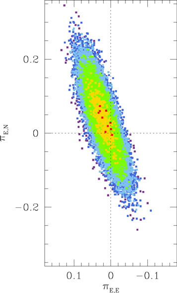
Figure 2. Distribution of Δχ2 in the (πE,N, πE,E) plane obtained from the analysis based on the ground-based data. Color coding indicates points in the MCMC chain within 1σ (red), 2σ (yellow), 3σ (green), 4σ (cyan), and 5σ (blue).
Download figure:
Standard image High-resolution image3.2. Additional Space-based Data
Knowing the difficulty of the secure πE measurement based on only the ground-based data, we test the possibility of πE measurement with the additional data obtained from Spitzer observations. To compute lensing magnifications seen from the Spitzer telescope, one needs the position and the distance to the satellite. The position of the Spitzer telescope was in the ranges of 110° ≲ R.A. ≲ 194° and −7° ≲ decl. ≲ 21° and the distance was in the range of 1.566 ≲ dsat/au ≲ 1.584 during the 2017 bulge season.
The Spitzer data partially covered the event light curve. Furthermore, they do not cover major features such as those produced by caustic crossings. See the Spitzer data presented in Figure 1. In such a case, external information of the color between the passbands used for observations from Earth and from the Spitzer telescope can be useful in finding a correct model (Yee et al. 2015; Shin et al. 2017). We, therefore, apply a color constraint with the measured instrumental color of I − L = 2.33 ± 0.012. The color constraint is imposed by giving penalty χ2 defined in Equation (2) of Shin et al. (2017).
For single-lensing events observed both from Earth and from a satellite, it is known that there exist four sets of degenerate solutions (Refsdal 1966; Gould 1994b). This degeneracy among these solutions, referred to as (+, +), (−, −), (+, −), and (−, +) solutions, arises due to the ambiguity in the signs of the lens-source impact parameters as seen from Earth (the former sign in parenthesis) and from the satellite (the latter sign in parenthesis). In many cases of binary-lens events, this four-fold degeneracy reduces into a two-fold degeneracy (Han et al. 2017) due to the lack of lensing magnification symmetry. The remaining two degenerate solutions, (+, +) and (−, −) solutions, are caused by the mirror symmetry of the source trajectory with respect to the binary axis, and thus the degeneracy corresponds to the "ecliptic degeneracy." Besides the known types, binary events can be subject to various other types of degeneracy.
In order to check the existence of degenerate solutions, we explore the space of the lensing parameters using two methods. First, we conduct a grid search over the (πE,N, πE,E) plane. Second, we search for local solutions using a downhill approach from various starting points that are obtained from the analysis based on the ground-based data. From these searches, we identify two classes of solutions, in which each class is composed of two solutions arising from the ecliptic degeneracy.
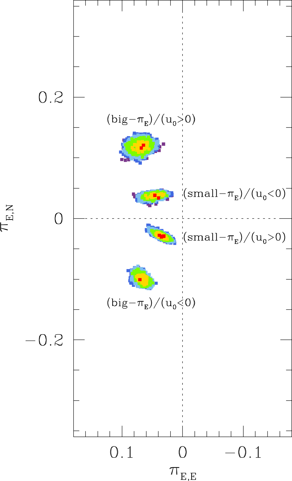
In Figure 3, we present the locations of the local solutions in the (πE,N, πE,E) plane. It is found that one pair of solutions has  ("big-πE" solutions) and the other pair has πE ≲ 0.1 ("small-πE" solutions). For each pair, the lensing parameters of the two degenerate solutions are approximately in the relation of
  , and thus we refer to the solutions as u0 < 0 and u0 > 0 solutions. We note that although the higher-order parameters (πE,N, πE,E, ds/dt, dα/dt) of these degenerate solutions are different from one another, the other lensing parameters are similar because they are mostly determined from the ground-based data. By comparing the ranges of the Δχ2 distributions with and without the Spitzer data, one finds that the uncertainties of the determined microlens-parallax parameters are greatly reduced with the use of the Spitzer data.

Figure 3. Distribution of Δχ2 in the (πE,N, πE,E) plane obtained from the analysis based on the ground+Spitzer data. Color coding is the same as that in Figure 2. The local minima indicate the positions of the four degenerate solutions.
Download figure:
Standard image High-resolution imageIn Table 3, we list the lensing parameters of the four degenerate solutions along with their χ2 values. We find that the (small-πE)/(u0 < 0) solution is preferred over the other solutions for two major reasons. First, the (small-πE)/(u0 < 0) solution provides a better fit to the observed data than the other solutions by 11.3 < Δχ2 < 25.3. Second, the small-πE solutions are preferred over the big-πE solution according to the "Rich argument" (Calchi Novati et al. 2015a), which states that, other factors being equal, small parallax solutions are preferred over large ones by a probability factor (πE,big/πE,small)2 ≳ 6. Although the (small-πE)/(u0 < 0) solution is favored, one cannot completely rule out the other degenerate solutions. We, therefore, discuss the methods that can firmly resolve the degeneracy in Section 5. Also presented in Table 3 are the fluxes of the source, fS,I, and the blend, fb,I, estimated based on the OGLE data. The small fb,I indicates that the blend flux is small. We note that the small negative blending is quite common for point-spread-function photometry in crowded fields (Park et al. 2004).
Table 3. Best-fit Parameters (with Spitzer Data)
| Parameter | Small πE | Big πE | ||
|---|---|---|---|---|
| u0 < 0 | u0 > 0 | u0 < 0 | u0 > 0 | |
| χ2 | 2373.1 (3.1) | 2398.4 (12.7) | 2395.1 (5.2) | 2384.4 (1.7) |
| t0 (HJD') | 7904.908 ± 0.098 | 7904.885 ± 0.106 | 7904.873 ± 0.057 | 7905.071 ± 0.057 |
| u0 | −0.151 ± 0.002 | 0.152 ± 0.002 | −0.151 ± 0.001 | 0.149 ± 0.001 |
| tE (days) | 41.73 ± 0.06 | 41.73 ± 0.05 | 41.71 ± 0.04 | 41.64 ± 0.04 |
| s | 1.438 ± 0.002 | 1.438 ± 0.002 | 1.440 ± 0.001 | 1.438 ± 0.001 |
| q | 0.704 ± 0.005 | 0.702 ± 0.006 | 0.701 ± 0.002 | 0.712 ± 0.003 |
| α (rad) | −0.642 ± 0.001 | 0.642 ± 0.001 | −0.648 ± 0.001 | 0.647 ± 0.001 |
| ρ (10−3) | 8.76 ± 0.07 | 8.69 ± 0.07 | 8.68 ± 0.05 | 8.78 ± 0.06 |
| πE,N | 0.034 ± 0.003 | −0.030 ± 0.004 | −0.100 ± 0.006 | 0.121 ± 0.007 |
| πE,E | 0.040 ± 0.009 | 0.031 ± 0.007 | 0.070 ± 0.007 | 0.065 ± 0.009 |
| ds/dt (yr−1) | 0.215 ± 0.058 | 0.197 ± 0.059 | 0.122 ± 0.013 | 0.175 ± 0.021 |
| dα/dt (yr−1) | −0.165 ± 0.031 | 0.158 ± 0.030 | −0.168 ± 0.020 | 0.009 ± 0.019 |
| fS,I | 7.35 | 7.36 | 7.37 | 7.35 |
| fb,I | −0.06 | −0.07 | −0.08 | −0.06 |
Note. The values in the parenthesis of the χ2 line represent the penalty χ2 values given by the color constraint. See more details in Section 3.2. HJD' = HJD−2450000.
Download table as: ASCIITypeset image
In Figure 4, we present the lens-system geometry of the four degenerate solutions. For each geometry, we present the source trajectories with respect to the lens components (small empty dots marked by M1 and M2) and the caustic (cuspy closed curve). For each geometry, the source trajectories seen from Earth and the Spitzer telescope are marked by blue and red curves (with arrows), respectively. We also present the portion of the light curve in the vicinity of the Spitzer data and the model light curve.

Figure 4. Lens system geometry and the portion of the light curve in the vicinity of the Spitzer data for the four degenerate solutions. For each lens system geometry, the source trajectories seen from Earth and the Spitzer telescope are marked by blue and red curves (with arrows), respectively. The cuspy closed curve represents the caustic. The coordinates are centered at the barycenter of the binary lens. The blue and red curves superposed on the data points represent the model light curves for the ground and Spitzer data, respectively.
Download figure:
Standard image High-resolution imageAs mentioned, the degeneracy between the u0 < 0 and u0 > 0 solutions is caused by the mirror symmetry of the lens system geometry. On the other hand, the degeneracy between the small-πE and big-πE solutions is caused by the difference in the source trajectory angles seen from the Spitzer telescope. For the small-πE solution, the source trajectory angle as seen from the Spitzer telescope is bigger than the angle of the source trajectory seen from the ground. In contrast, the Spitzer trajectory angle of the big-πE solution is smaller than the angle of the ground trajectory. We note that the latter degeneracy is different from the degeneracy between (+, +) and (+, −) solutions because both ground and satellite trajectories pass on the same side with respect to the barycenter of the binary lens. Such a degeneracy is not previously known.
In order to further investigate the cause of the degeneracy between the small-πE and big-πE solutions, in Figure 5, we present the magnification contours in the outer region of the caustic. On the contour map, we plot the Spitzer source trajectories of the two degenerate solutions. From the map, it is found that the magnification patterns along the source trajectories of the two degenerate solutions are similar to each other, suggesting that the degeneracy is caused by the symmetry of the magnification pattern in the outer region of the caustic. We note that the degeneracy could have been resolved if the caustic exit part of the light curve had been covered by Spitzer data because the times of the caustic exit (seen from the Spitzer telescope) expected from the two degenerate solutions are different from each other. We find that the caustic exit times for the small-πE solutions are in the range of 7926 (for u0 < 0) ≲ HJD' ≲ 7928 (for u0 > 0). On the other hand, the range for the big-πE solutions is 7922 (for u0 < 0) ≲HJD' ≲ 7924 (for u0 > 0). With the ∼4 day time gap between the caustic-crossing times of the small-πE and big-πE solutions, the degeneracy could have been easily lifted. In conclusion, we find that the new type of degeneracy is caused by the partial symmetry of the magnification pattern outside the caustic combined with the fragmentary coverage of the Spitzer data.

Figure 5. Contour map of lensing magnification in the outer region of the caustic. Contours are drawn at every ΔA = 0.05 step from A = 1.1 to A = 2.0. The lines with arrows represent the source trajectories of the small-πE and big-πE solutions seen from the Spitzer telescope. The crosses on each trajectory represent the expected positions of the source when Spitzer data were taken.
Download figure:
Standard image High-resolution imageFrom the comparison of the analyses conducted with and without the space-based data, we find two important results.
- 1.First, while the microlens parallax cannot be securely determined based on only the ground-based data, the addition of the Spitzer data enables us to clearly identify two classes of microlens-parallax solutions. The degeneracy is either intrinsic to lensing systems (u0 < 0 versus u0 > 0 degeneracy) or due to the combination of the partial symmetry of the magnification pattern combined with the fragmentary Spitzer coverage of the event (small-πE versus big-πE degeneracy).
- 2.Second, the space-based data greatly improve the precision of the πE measurement. We find that the measurement uncertainties of the north and east components of
 are reduced by factors of ∼18 and ∼4, respectively, with the use of the Spitzer data. Since the lens mass is directly proportional to 1/πE, the uncertainty of the mass measurement reduces by the same factors.

4. Physical Lens Parameters
4.1. Source Star and Angular Einstein Radius
For the unique determination of the lens mass and distance, one needs to estimate the angular Einstein radius in addition to the microlens parallax. Since the angular Einstein radius is determined by θE = θ*/ρ, it is required to estimate the angular radius of the source star.
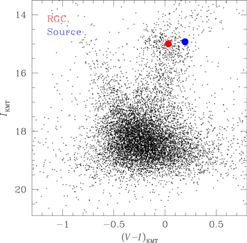
We estimate θ* from the dereddened color (V − I)0 and brightness I0 of the source. In order to derive (V − I)0 from the instrumental color–magnitude diagram, we use the method of Yoo et al. (2004), which uses the centroid of the red giant clump (RGC) as a reference. In Figure 6, we present the location of the source and the RGC centroid in the instrumental color–magnitude diagram constructed from the I- and V-band DoPHOT photometry of the KMTC data set. It is found that the offsets in color and brightness of the source with respect to the RGC centroid are Δ(V − I, I) = (0.16, −0.07). With the known dereddened color and magnitude of RGC centroid, (V − I, I)RGC = (1.06, 14.5) (Bensby et al. 2011; Nataf et al. 2013), we find that the dereddened color and brightness of the source star are (V − I, I)0 = (V − I, I)RGC + Δ(V − I, I) = (1.22 ± 0.07, 14.48 ± 0.09). This indicates that the source is a K-type giant star. Using the color–color relation provided by Bessell & Brett (1988), we convert V − I into V − K. Using the relation between V − K and the surface brightness (Kervella et al. 2004), we estimate the angular source radius. The estimated angular source radius is θ* = 6.9 ± 0.6 μas. Combined with the value of ρ, we estimate that the angular Einstein radius of the lens system is

With the measured angular Einstein radius, the relative lens-source proper motion is estimated by

Figure 6. Location of the source with respect to the centroid of the red giant clump (RGC) in the instrumental color–magnitude diagram.
Download figure:
Standard image High-resolution image
4.2. Lens Parameters
With the measured microlens parallax and the angular Einstein radius, we estimate the mass and distance to the lens using the relations in Equation (2). For this, we estimate the distance to the source by  where DGC = 8.16 kpc is the distance to the galactic center (Nataf et al. 2013), l = −254 is the galactic longitude of the source, and ϕ = 40° is the orientation angle of the bar-shaped bulge with respect to the line of sight. This results in DS = 8.62 kpc and πS = 0.116 mas. In Table 4, we list the determined physical parameters, including masses of the primary, M1, and the companion, M2, the distance to the lens, DL, and the projected separation between the lens components, a⊥ = sDLθE, for the individual degenerate lensing solutions. To check the physical validity of the parameters, we also present the ratio between the projected potential energy to the kinetic energy, i.e., (KE/PE)⊥.
Table 4. Physical Lens Parameters
| Parameter | Small πE | Big πE | ||
|---|---|---|---|---|
| u0 < 0 | u0 > 0 | u0 < 0 | u0 > 0 | |
| M1 (M⊙) | 1.09 ± 0.15 | 1.33 ± 0.21 | 0.47 ± 0.04 | 0.41 ± 0.04 |
| M2 (M⊙) | 0.77 ± 0.11 | 0.93 ± 0.15 | 0.33 ± 0.03 | 0.29 ± 0.03 |
| DL (kpc) | 6.38 ± 0.79 | 6.66 ± 0.86 | 4.69 ± 0.45 | 4.48 ± 0.42 |
| a⊥ (au) | 7.20 ± 0.89 | 7.59 ± 0.98 | 5.35 ± 0.52 | 5.04 ± 0.47 |
| (KE/PE)⊥ | 0.12 ± 0.02 | 0.12 ± 0.02 | 0.09 ± 0.01 | 0.04 ± 0.01 |
| ψ (deg) | 51 | 132 | 141 | 32 |
Download table as: ASCIITypeset image
Due to the difference in the microlens-parallax values between the small-πE and big-πE solution classes, the estimated lens masses and distances for the two classes of solutions are substantially different from each other. On the other hand, the physical parameters for the pair of the u0 > 0 and u0 < 0 solutions are similar to each other. We find that the masses of the primary and companion are 1.1 ≲ M1/M⊙ ≲ 1.3 and 0.8 ≲ M2/M⊙ ≲ 0.9 for the small-πE solutions. For the big-πE solutions, the masses of the lens components are 0.4 ≲ M1/M⊙ ≲ 0.5 and M2 ∼ 0.3 M⊙. The estimated distances to the lens are 6.4 ≲ DL/kpc ≲ 6.7 and 4.5 ≲ DL/kpc ≲ 4.7 according to the small-πE and big-πE solutions, respectively.
5. Resolving Degeneracy
5.1. Lens Brightness
The estimated masses of the lens for the small-πE and big-πE solutions are considerably different due to the difference in the measured microlens-parallax values. Then, if the lens-source can be resolved from future high-resolution imaging observations, the degeneracy can be resolved from the lens brightness.
If the proposed follow-up high-resolution observations are conducted, the observations will likely be conducted in the near-IR band. We, therefore, estimate the H-band magnitudes of the source and lens. From the dereddened I-band magnitude I0 ∼ 14.5, the dereddened H-band source magnitude of the source is H0 ∼ 13.1 (Bessell & Brett 1988). The V-band extinction of AV ∼ 2.6 in combination with the extinction ratio (AH/AV) ∼ 0.108 (Nishiyama et al. 2008) toward the bulge field yields the H-band extinction of AH ∼ 0.28. Then, the apparent H-band magnitude of the source is HS = H0 + AH ∼ 13.4. We compute the lens brightness based on the mass and distance under the assumption that the lens and source experience the same amount of extinction. In Table 5, we present the expected combined (primary plus companion) I- and H-band magnitudes of the lens and source. The brightness of the lens varies depending on the solution. For the small-πE solutions, the apparent H-band magnitude of the lens is HL ∼ 16.5–17.0. For the big-πE solutions, on the other hand, the expected H-band lens brightness is HL ∼ 18.7–19.1.
Table 5. Expected Lens Brightness
| Solution | Lens | Source | |||
|---|---|---|---|---|---|
| IL | HL | IS | HS | ||
| Small πE | u0 < 0 | 18.8 | 17.0 | 15.8 | 13.5 |
| u0 > 0 | 17.7 | 16.5 | ⋯ | ⋯ | |
| Big πE | u0 < 0 | 21.5 | 18.7 | ⋯ | ⋯ |
| u0 > 0 | 22.1 | 19.1 | ⋯ | ⋯ | |
Download table as: ASCIITypeset image
According to the estimated I-band lens brightness, the lens-to-source flux ratio for the (small-πE)/(u0 > 0) solution is fL,I/fS,I ∼ 17%. Since the light from the lens contributes to blended light, then, this ratio is too big to be consistent with the small amount of the measured blended flux, even considering the uncertainties of the lens mass and distance. Therefore, the solution is unlikely to be the correct solution not only because of its worst χ2 value among the degenerate solutions but also because of the limits on blended light. The lens-to-source flux ratio for the (small-πE)/(u0 < 0) is about 6%, but with the lens mass and distance at the 1σ (2σ) level, the ratio is ∼2% (1%), which is consistent with the blending.
5.2. Relative Lens-source Proper Motion
The degeneracy between u0 < 0 and u0 > 0 solutions can also be lifted once the lens and source are resolved. The relative lens-source proper motion vector is related to tE, θE, and (πE,N, πE,E) by

For the pair of the degenerate solutions with u0 < 0 and u0 > 0, the north components of  have opposite signs. This implies that the relative motion vectors of the two degenerate solutions are directed in substantially different directions and thus the degeneracy can be resolved from the lens motion with respect to the source.
The heliocentric lens-source proper motion is μhelio ∼ 7 mas yr−1, which is about what is expected for a disk lens. In this case, the expected direction of  (i.e., the direction of Galactic rotation ψ ∼ 30°) is roughly 30° east of north. In Table 4, we list the orientation angles ψ of
  , as measured from north to east, corresponding to the individual solutions. The heliocentric proper motion is related to the geocentric proper motion
  by
by

where v⊕,⊥ represents the projected Earth motion at t0. One finds that the expected direction  is consistent with the (small-πE)/(u0 < 0) and the (big-πE)/(u0 > 0) solutions but inconsistent with the others.
From Keck adaptive optics observations, Batista et al. (2015) resolved the lens from the source ∼8.2 years after the event OGLE-2005-BLG-169, for which the relative lens-source proper motion is μ ∼ 7.4 mas yr−1. The estimated proper motion of OGLE-2017-BLG-0329 (μ ∼ 6.9 mas yr−1) is similar to that of OGLE-2005-BLG-169. Considering the large lens/source flux ratio, the lens-source resolution by Keck observations will take ∼10 years, which is somewhat longer than the time for OGLE-2005-BLG-169. We note that GMT/TMT/ELT, which will have better resolution than Keck, may be available before Keck can resolve the event and thus the time for follow-up observations can be shortened.
6. Conclusion
We presented the analysis of the binary microlensing event OGLE-2017-BLG-0329, which was observed both from the ground and in space using the Spitzer telescope. We found that the parallax model based on the ground-based data could not be distinguished from a zero-πE model at the 2σ level. However, with the use of the additional Spitzer data, we could identify two classes of microlens-parallax solutions, each composed of a pair of solutions according to the well-known ecliptic degeneracy. We also found that the space-based data helped to greatly reduce the measurement uncertainties of the microlens-parallax vector  . With the measured microlens parallax combined with the angular Einstein radius measured from the resolved caustics, we found that the lens was composed of a binary with component masses of either (M1, M2) ∼ (1.1, 0.8) M⊙ or ∼(0.4, 0.3) M⊙ according to the two solution classes. The degeneracy among the solution would be resolved from adaptive optics observations taken ∼10 years after the event.
Work by C. Han was supported by the grant (2017R1A4A1015178) of the National Research Foundation of Korea. Work by W.Z., Y.K.J., and A.G. was supported by AST-1516842 from the US NSF. W.Z., I.G.S., and A.G. were supported by JPL grant 1500811. The OGLE project has received funding from the National Science Centre, Poland, grant MAESTRO 2014/14/A/ST9/00121 to A.U. Work by Y.S. was supported by an appointment to the NASA Postdoctoral Program at the Jet Propulsion Laboratory, administered by Universities Space Research Association through a contract with NASA. This work was (partially) supported by NASA contract NNG16PJ32C. Work by S.R. and S.S. is supported by INSF-95843339. This research has made use of the KMTNet system operated by the Korea Astronomy and Space Science Institute (KASI) and the data were obtained at three host sites of CTIO in Chile, SAAO in South Africa, and SSO in Australia. We acknowledge the high-speed internet service (KREONET) provided by Korea Institute of Science and Technology Information (KISTI).