First Thomson scattering results from AWAKE's helicon plasma source

The helicon plasma source (HPS) for AWAKE was originally developed at the Max Planck institute for Plasma Physics (IPP) in Greifswald, Germany, and characterized with a CO₂ interferometer, as reported in [28]. After demonstrating the nominal AWAKE density of 7$\times 10^{-20}$ m⁻³, the system was reinstalled at CERN with some improvements. We will shortly describe the plasma source itself, the changes implemented at CERN and the operating parameters anticipated to generate highest densities as found in [28].

The plasma is generated in a 1 m long quartz tube with 44 mm inner diameter, equipped with three optical view ports, as shown in figure 1. The axial magnetic field B₀ of up to 125 mT is provided by a DC current of $\unicode{x2A7D}$400 A through five water-cooled copper coils. Three RF antennas are equidistantly (230 mm) distributed along the quartz tube and over the view ports and fed by three individual RF power supplies delivering $P_\textrm{RF} \unicode{x2A7D}$ 12 kW per antenna.

Zoom In Zoom Out Reset image size

The RF generators are operated at $f_\textrm{RF} =$ 13.56 MHz. They are run in a ramp-up sequence with six individual pulses, the last three reaching the nominal power. The pulses are generated at a frequency of 10 Hz with a fast (2 µs) rise time and a pulse duration of 5 ms, each. Due to the long separation (100 ms) between the single RF pulses, the plasma generated in each pulse can be regarded as independent of the other pulses. The ramp-up sequence was necessary only due to technical constraints of the RF generators. To limit the heat load on the antennas and the vacuum chamber, the RF sequence is repeated every 5 s, resulting in an effective operation frequency of 0.2 Hz, as illustrated in figure 2. Each RF generator is coupled to its antenna by a manual floating L-type capacitive matching circuit to minimize reflected power. The matching is adjusted to the steady-state plasma conditions. Each time the experimental parameters (in particular DC magnetic field and RF power) are changed, the matching is adjusted accordingly. The relative phase of the RF field provided to the three antennas can be controlled at the RF power supplies that are operated with the same master clock. Note that the phase relation between the antennas can strongly affect the matching network and the achieved plasma parameters.

Zoom In Zoom Out Reset image size

During reinstallation of the HPS at CERN several experimental details were altered compared to the previous setup operated at IPP Greifswald. In the initial setup [28], 75-mm-long half-helical antennas generating m = 1 modes were employed. With this setup, no resonant effects were observed. In particular, the electron density that is expected to dominantly propagate a helicon wave at the same wavelength as the half-helical antenna, was not generated preferentially. Consequently, we have opted to replace the original antennas with m = 0 mode ring antennas that provide several advantages. (i) The 10-mm-wide copper rings can be easily fabricated and installed on the HPS. (ii) The m = 0 mode promotes symmetric plasma generation in both, the upstream and downstream directions. (iii) The cross-talk between antennas, where one receives the RF field generated by the others, is reduced due to a smaller effective surface area and the larger effective inter-antenna distance. Furthermore, the pumping scheme of the HPS was changed from pumping and gas feed being situated at opposite sides of the quartz tube (steady-state flow) to a scheme where they are installed on the same side (resulting in an almost stationary gas situation). The previously employed pump was exchanged by a turbo molecular pump and a scroll pump to achieve a lower base pressure. Additionally, adaptation to the CERN laboratory required the modification of the grounding scheme of the HPS, as well as utilization of longer RF cables and different positions of DC ceramic breakers at the ends of the vacuum chamber.

The HPS is operated with argon due to its relatively low ionization energy of 15.76 eV, its inert chemical character and its good availability. The pressure is adjusted to a few (5 – 10) Pa, typically, such that the nominal AWAKE density can be achieved at an ionization degree of 0.25 – 0.5. Furthermore, a simple power and particle balance model (PPM) [29] showed that with a power of ≈30 kW the required density can be achieved with $T_e \lt$ 2 eV. Indeed, in [28], the nominal AWAKE density of 7$\times 10^{-20}$ m⁻³ was achieved for $P_\textrm{RF} =$ 27 kW, delivered by three antennas (9 kW/antenna), at $p =$ 8 Pa and $B_0 =$ 106 mT. The RF phase between the single antennas was adjusted at the RF source to be 180:270:0 for antennas 1:2:3.

A new TS diagnostics was installed to measure the local electron density n_e and temperature T_e, and to benchmark the HPS operation after reinstallation at CERN The TS system was developed on the Resonant Antenna Ion Device (RAID) [19] at EPFL as improvement of a previous diagnostics [27]. Using the second harmonic of the Nd:YAG laser allowed us to replace the polychromator and avalanche photo diodes by a spectrometer and a gated ICCD camera, as demonstrated in [30]. Furthermore, the shorter wavelength guarantees that the diagnostic is operating in the incoherent TS regime for the expected HPS densities. The setup is described in detail in the following.

The TS setup relies on the second harmonic of a Quantel Brilliant $B, Q$-switched Nd:YAG laser with an energy of 350 mJ/pulse at 532 nm. The laser operates at 10 Hz with a pulse width of 7 ns. The 8 mm-diameter laser beam is focused into the vacuum quartz tube along the axis by a f = 1200 mm lens. A Brewster window and a set of five diaphragms with aperture varying between 9 mm and 7 mm diameter have been installed at the entrance and at the exit of the quartz tube to reduce laser stray light. The focal spot size of the laser pulse is approximately 2 mm in diameter. The scattered light is collected through the view port 2 at z = 50 cm, in the center of the quartz tube. Reflections from the opposite side of the port at the laser wavelength are significantly reduced by a CuO coating. An $f =$ 20 mm, d = 25 mm aspheric lens is used to image a 4 mm diameter plasma section into a 910 µm optical fiber. The collection volume is, therefore, $\approx 2 \times 2 \times 4$ mm³ and defines the spatial resolution of the measurements. A polarizer is inserted in the collection path to reduce the recorded plasma self-emission. In order to suppress stray light from reflections and Rayleigh scattering, a filter setup based on a volume Bragg grating from OptiGrate, providing a band-width of 0.3 nm with an optical density OD = 4 [31, 32], is used. The light exiting the fiber is collimated using a $d =$ 50 mm, f = 100 mm aspheric lens. In the present setup, the collimation of the light from the 910 µm fiber is not sufficient to reach the specified extinction of OD 4. However, this approach was chosen as a compromise between simple implementation of the optics, optical throughput, and filtering performance. The filtered light is imaged by an f = 75 mm spherical lens onto the input slit of a high through-put f/2, f = 200 mm lens based (Nikon AI 200 mm f2 ED IF) spectrometer, that is equipped with a 2400 l/mm grating. The spectrometer is coupled to a Princeton Instruments PiMax (PM4-1024f-SR-FG-18-P43) gated Intensified Charged Coupled Device (ICCD). The typical gate time is adjusted to 30 ns to record the entire laser pulse and to account for a jitter of ≈8 ns in the trigger chain. The system provides a dispersion of δλ = 0.024 nm/px. High-resolution measurements with entrance slit width of 200 µm yield a spectral resolution of Δλ = 0.13 nm. To increase the optical throughput, measurements are typically taken with a 500-µm entrance slit with Δλ = 0.4 nm (flat-top). To achieve an acceptable signal-to-noise ratio (SNR), measurements are averaged over 50 to 200 laser pulses. With the HPS operating at 0.2 Hz, this results in an effective measurement time of four to 16 min per spatial and temporal point. During the measurement time, the experimental conditions, e.g. the RF power $P_\textrm{RF}$, the argon pressure p, and the DC magnetic field B₀, exhibit a variation of less than ± 2.5%. The uncertainty due to the shot-to-shot reproducibility of the experimental parameters during one measurement is well below the statistical uncertainty of the analysis (see section 3.1). Furthermore, the laser intensity is monitored by a fast photo-diode that records a diffuse reflection from one of the mirrors and the obtained TS signal is corrected for potential variations.

The TS setup described above enables the precise, local measurement of n_e in the HPS, and furthermore provides a measurement of the electron temperature T_e, that was previously inaccessible. Figure 3 illustrates the TS measurement obtained with a spectrometer entrance slit of 500 µm and averaged over 100 laser pulses. The data have been acquired at the fifth RF pulse, see figure 2, with $P_\textrm{RF}$ = 27 kW (9 kW/antenna), $p = 8~$Pa Argon, B₀ = 106 mT, and at $t\,= ~{350}$ µs after the start of the RF pulse. The data have been corrected for electronic background noise, residual stray light at the laser wavelength, and emission from the plasma. The recorded spectrum has been fitted with a Gaussian distribution function, where the data shown in gray are excluded from the fit. The central region at 532 nm is not taken into account due to remaining laser stray light and distortion effects from the notch filter. The region at 528.7 nm is excluded due to intensity fluctuations of the plasma self emission resulting from the Ar II 4 s - 4p transition. Shown are the best fit as red solid line, as well as the uncertainties from the fit accounting for 1-σ in red dashed and dotted lines. In the example shown, the FWHM of 3.47 nm yields an electron temperature of T_e = 2.0 eV. The scattered intensity was absolutely calibrated using Raman scattering in nitrogen and yields an electron density of n_e = 2.6$\times 10^{-20}$ m⁻³.

Zoom In Zoom Out Reset image size

The uncertainty of the TS measurement can be estimated as follows. For T_e, the statistical uncertainty from the Gaussian fit (3-σ) accounts for typically ±0.1 eV. An uncertainty in the dispersion of 0.002 nm/px causes a systematic error in T_e of 1%, which is negligible in comparison to the statistical uncertainty. For n_e, the statistical uncertainty due to the Gaussian fit is 7%. Additionally, several sources of uncertainty from the absolute calibration have to be taken into account: 1) the reproducibility of the laser energy introduces a statistical uncertainty of 2.5%; 2) the pressure of the N₂ gas used for the calibration was determined with an accuracy of 3%; 3) the theoretical Raman cross sections are known to a precision of 8% [33]; 4) the measured Raman spectrum can be fitted to a precision of 5%; 5) the polarization purity of the laser pulse (≈80%) can induce an uncertainty of up to 5% and leads to an underestimation of the measured electron density. Considering all sources of error to be independent, we can use Gaussian error propagation. Therefore, the statistical uncertainty of n_e accounts for 8.5% while the systematic uncertainty (which is the same for all measurements taken with the same calibration) is −11% and +10%.

Figure 4 illustrates the time evolution of the electron density (black symbols) and of the temperature (red symbols) at the center of the HPS for operation parameters $P_\textrm{RF}$ = 12 kW (4 kW/antenna), p= 8 Pa argon, and B₀ = 106 mT. During the first 100 µs after the start of the fifth RF pulse, the electron density is below the sensitivity of the TS diagnostics. Subsequently, n_e increases rapidly to ≈1.6$\times 10^{-20}$ m⁻³ at t = 200 µs. The peak density of 1.9$\times 10^{-20}$ m⁻³ is reached at $t =$ 350 µs and remains approximately constant until $t =$ 1000 µs. The electron temperature ranges between 1.5 eV, at the beginning of the discharge, and increases up to 2.2 eV. At the time of peak density, the electron temperature is typically around 2.0 eV. The minor variation of the plasma parameters after t = 350 suggests that a stable plasma condition is reached and that the plasma can be modeled by a steady-state approximation. Note that the temporal evolution of the plasma parameters changes slightly with the experimental parameters (B-field, power, pressure). In the following, data obtained at the time of peak density, typically between $t = {300}\,\mu$s and $t = {350}\,\mu$s, are presented.

Zoom In Zoom Out Reset image size

The effect of the argon pressure on the plasma parameters in the investigated pressure range is illustrated in figure 5. The presented data indicate a rather small effect of the background gas pressure on the electron density at the center of the plasma column. In contrast, a significant decrease of electron temperature with increasing pressure is observed, which is consistent with the predictions from global 0D models [29, 34] and will be further discussed in section 5.1.

Zoom In Zoom Out Reset image size

In contrast to pressure, the magnetic field has a large impact on the electron density, as shown in figure 6 for constant power and pressure of 27 kW (9 kW/antenna) and 8 Pa, respectively. For B₀ up to ≈106 mT, the electron density appears to increase linearly with magnetic field, while at larger field amplitude the density saturates. This correlation was also observed previously [28] and attributed to the classical dispersion relation of helicon waves [35],

$$\begin{equation} \omega = \frac{k k_{\parallel}}{q \ \mu_0} \frac{B_0}{n_e} ,\end{equation} \tag{ 1 }$$

where ω is the wave's angular frequency, k and $k_{\parallel}$ are the norms of the total and the parallel (to the DC magnetic field) wave vectors, respectively, q is the electron charge, and µ₀ the vacuum permeability. For a wave excitation at constant frequency $f = \omega/2\pi$ at 13.56 MHz, the electron density is proportional to the magnetic field, given that the wave configuration, $k k_{\parallel}$, is constant. This relation holds as long as the helicon wave frequency is larger than the lower hybrid frequency $\omega \gt \omega_\textrm{LH} \approx \sqrt{\omega_{ce} \omega_{ci}}$, where ω_ce and ω_ci are the electron and ion cyclotron frequencies, respectively. For a driving frequency of 13.56 MHz, ω_LH is reached at a magnetic field as high as 132 mT, which could, therefore, explain the flattening of the density curve at large B-fields. However, applying the helicon approximation to the present experiment is clearly an oversimplification of the system (perfectly conducting boundary, homogeneous electron density, no collisions). Moreover, previous results showed that in case of a weakly bounded helicon plasma, the axial wavelength is not constant but adjusts smoothly to the applied B-field and density [36]. In this case, the geometric configuration of the experiment is clearly not imposing the wave vector geometry ($k k_{\parallel} = \textrm{const}$) of the helicon wave.

Zoom In Zoom Out Reset image size

The variation of the plasma parameters with the power delivered to each antenna is illustrated in figure 7. The power was varied from 4 kW/antenna to 9 kW/antenna and the matching network of the three antennas was optimized individually for each power. Note that the data presented in figures 7 and 6 were obtained several months apart from each other. Consequently, additional changes in the HPS setup had a discernible impact on the absolute electron density. Nonetheless, the trends depicted remain valid. Figure 7 shows that the electron temperature is rather constant over the probed power range, while the electron density increases slightly. In particular, a doubling of the RF power results in an increase of the electron density of 25% from 2$\times 10^{-20}$ m⁻³ to 2.5$\times 10^{-20}$ m⁻³. The rather moderate increase of density at this high power level might be related to the phenomenon of neutral depletion [37], which may affect the plasma density at ionization degrees as low as 1%. Further investigation of the transport of ions and neutrals, for example by LIF [24], is highly desired to understand the impact of these phenomena on the HPS. Additional effects potentially related to a flattening of the electron density will be discussed in section 5.3.

Zoom In Zoom Out Reset image size

In order to simulate the propagation of the helicon wave in plasma and deduce its power density, we solve Maxwell's equations with a time harmonic ansatz $\vec{X}(\vec{r},t) = \vec{X}(\vec{r})\textrm{e}^{-\textrm{i} \omega t}$ and describe the plasma medium by a complex conductivity tensor.

Using the time harmonic ansatz, Maxwell's equations can be combined to yield the wave equation

$$\begin{equation} \vec{\nabla} \times \vec{\nabla} \times \vec{E} = \mu_0 \omega^2 \boldsymbol{\epsilon} \vec{E} ,\end{equation} \tag{ 2 }$$

where $\boldsymbol{\epsilon}$ is the complex dielectric tensor describing the response of the plasma. A constitutive relation for the plasma medium (Ohm's law) can be found from the first moment of Boltzmann's equation (momentum conservation) for the electron fluid:

$$\begin{equation} m_e \partial_t \vec{u} + q \vec{E} + q \vec{u} \times \vec{B}_0 + \nu_{en} m_e \vec{u} = 0 ,\end{equation} \tag{ 3 }$$

where $\vec{u}$ represents the mean fluid velocity, m_e the electron mass, $\vec{E}$ the oscillating electric field, $\vec{B}_0$ the background magnetic field aligned to the z-direction, and ν_en the effective electron-neutral collision frequency. Equation (3) represents a classical, collisional model that is equivalent to the concept of Ohmic heating. Defining the current density as $\vec{j} = -q n_e \vec{u}$ and using the time harmonic ansatz, we can re-write equation (3) as

$$\begin{equation} \vec{E} = \frac{1}{\epsilon_0 \omega_{pe}} \left[ \hat{\omega} \vec{j} + \omega_{ce} \vec{j} \times \vec{e}_z \right] ,\end{equation} \tag{ 4 }$$

where we introduce the plasma angular frequency of electrons $\omega_{pe} = \sqrt{q^2 n_e / \epsilon_0 m_e}$, the electron cyclotron frequency $\omega_{ce} = q B_0 / m_e$, and the complex frequency $\hat{\omega} = \nu_{en} - i \omega$. Note, that we did not use the approximations common in helicon physics to derive equation (4). In particular, we did not assume a constant electron density, perfectly conducting boundaies, or negligible collisionality. Accordingly, we can estimate the power deposition into the plasma due to the collisions.

Equation (4) is equivalent to Ohm's law $\vec{j} = \boldsymbol{\sigma} \vec{E}$ with the complex conductivity tensor

$$\begin{equation} \boldsymbol{\sigma} = \frac{\epsilon_0 \omega^2_{pe}}{\hat{\omega}^2 + \omega_{ce}^2} \begin{pmatrix} \hat{\omega} & -\omega_{ce} & 0 \\ \omega_{ce} & \hat{\omega} & 0 \\ 0 & 0 & \left(\hat{\omega}^2 + \omega_{ce}^2\right) / \hat{\omega} \end{pmatrix} ,\end{equation} \tag{ 5 }$$

which yields the complex dielectric tensor

$$\begin{equation} \boldsymbol{\epsilon} = \epsilon_0 \left[ 1 + \frac{\boldsymbol{\sigma}}{-\textrm{i} \omega \epsilon_0} \right].\end{equation} \tag{ 6 }$$

Inserting equation (5) into equation (2), the wave equation is solved numerically. Therefore, the detailed HPS geometry was modeled in COMSOL [38] electromagnetic module and an initial electron density, shown in figure 8 a, was defined. For our convenience, we impose a radial electron density profile throughout this paper that follows the power law

$$\begin{equation} n_e\left(r\right) = n_0 \left( 1 - \frac{r^{\,n}}{R_p^n} \right) ,\end{equation} \tag{ 7 }$$

where R_p is the radius of the plasma boundary and n₀ the electron density on-axis. This electron density profile can easily be integrated radially and allows to establish a simple expression for the following 1D PPM. In the present work, we set n = 2 to achieve a parabolic density profile. In axial direction, the initial electron density distribution is defined as flat, $n_0(z) =$const, and to fall off parabolically at the boundary.

Zoom In Zoom Out Reset image size

The principal output of the wave calculation further used for the PPM is the deposited power mapping, generally expressed as:

$$\begin{equation} Q_\textrm{wave}\left(r,z\right) = \frac{1}{2} \left[ \vec{j}^* \cdot \vec{E} + \vec{j} \cdot \vec{E}^* \right].\end{equation} \tag{ 8 }$$

It was found in 3D calculations, performed with a ring antenna configuration, that the resulting wave presents a very clear m = 0 feature with azimuthal invariance. We, therefore, switch to a 2D calculation that provides a higher precision, as it allows for a denser mesh than in the 3D simulation. The results of this 2D simulated power deposition are shown in figure 8. Figure 8(a) illustrates the initial electron density map with a peak value $n_0 =$ 2.6$\times 10^{-20}$ m⁻³ at a background gas pressure of 8 Pa. In figure 8(b) we show the resulting 2D power deposition for a single antenna. The power transfer efficiency to the plasma, accounting for the resistance of the antenna, was considered and found to be $\unicode{x2A7E}$80%. The power deposition profile is axially symmetric around the antenna position, as expected for an m = 0 ring antenna, and exhibits an axial wavelength of ≈5 cm. The radial profile changes drastically with the distance from the antenna. At the antenna position, the main power is deposited close to the plasma edge by modes that are characterized by short radial (and axial) wavelengths, as well as strong radial damping. These modes can be identified as belonging to the Trivelpiece-Gould (TG) family [39]. Further away from the antenna, the power deposition peaks on-axis, due to dominant helicon H-modes that are characterized by a radial wavelength comparable to the radius of the vacuum tube.

In figure 8(c) we extend the calculation to the actual geometry of the HPS with three antennas. The interaction of the antennas with each other manifests itself in the development of distinct interference patterns. At the antenna positions, increased power deposition at the outer plasma boundary is observed, as expected from the 1-antenna calculation. Additionally, the waves propagating from the neighboring antennas lead to some power deposition also on-axis at the antenna positions. Asymmetries in the axial directions are caused by the lack of symmetry in the boundary conditions of the present setup of the HPS.

After we have calculated the power deposited by the helicon wave, we can use a PPM to evaluate the resulting electron density n_e and temperature T_e. We use here $Q_\textrm{wave}$ as a source for the electron fluid temperature, and, as a consequence, for ionization. This source of particles and power is balanced by the losses of the charged particles and their associated energy at the plasma boundary. We, therefore, need to evaluate the particle's energy and flux (perpendicular to the boundary) at the boundary. In axial direction, we use the model of ambipolar diffusion, where the particle flux results from the fluid equations. In radial direction, we employ a floating sheath model that defines the particle density and velocity at the sheath entrance. We can then solve the particle and the power balance equations to find the 1D steady-state axial profiles of n_e and T_e.

We consider the particle flux $\vec{\Gamma} = n\vec{u}$

$$\begin{equation} \vec{\nabla} \cdot \vec{\Gamma} = k_i\left(T_e\right) n_g n_e ,\end{equation} \tag{ 9 }$$

where the source term is due to electron impact ionization with k_i the (strongly dependent on electron temperature) rate coefficient for ionization and n_g the neutral gas density.

In axial direction, we consider a particle flux $\Gamma_z$ due to ambipolar diffusion, so that $\Gamma_z = - \mu_i \partial_z p_e$, where we assume that the ion temperature T_i and the ion mobility µ_i are much smaller than their electronic counterparts T_e and µ_e: $T_i \ll T_e$ and $\mu_i = q / m_i \nu_{in} \ll \mu_e = q / m_e \nu_{en}$ [34]. Both, ions and electrons, are, therefore, moving at the same velocity and $\vec{\Gamma}_i = \vec{\Gamma}_e = \vec{\Gamma}$. Here, $m_{i,e}$ is the mass of electrons and ions and $\nu_{in,en}$ is their effective collision frequency with neutrals. At the boundary (z = 0 and z = 1 m) of the simulation domain, the losses are defined by the particle flux at the sheath entrance $\Gamma_{z}(0) = \Gamma_{z}(1) = n_\textrm{sh} u_\textrm{Bohm}$ [40], given by the particle density at the sheath entrance $n_\textrm{sh} = n_0 \textrm{e}^{-1/2}$ and the Bohm velocity $u_\textrm{Bohm} = \sqrt{{q T_e}/{m_i}}$, where T_e is given in Volt.

In order to describe the losses in radial direction, the sheath model has to be modified due to the presence of the magnetic field that confines the particles to some degree. Therefore, we introduce the screening factor, $f_{\xi} \lt 1$, to account for the reduction of the radial transport and of particle losses [40]

$$\begin{align} \Gamma_r\left(R_p\right) & = n^{B_0}_\textrm{sh} \ u^{B_0}_\textrm{sh} = f_{\xi} \ n_\textrm{sh} \ u_\textrm{Bohm} \nonumber\\ & = f_{\xi} \ n_0 \textrm{e}^{-1/2} \ \sqrt{\frac{q T_e}{m_i}} .\end{align} \tag{ 10 }$$

We can now integrate over the particle flux using Gauss' divergence theorem

$$\begin{equation} \int_{\Delta S} \vec{\Gamma} \vec{\textrm{d}S} \ = \int_{\Delta V} \vec{\nabla} \cdot \vec{\Gamma} \textrm{d}V = \ \int_{\Delta V} k_i n_g n_e \textrm{d}V \ .\end{equation} \tag{ 11 }$$

The integration volume is the cylindrical elementary volume $\Delta V = \int_0^{2\pi} \int_0^{R_p} \int_z^{z+\Delta z} r \textrm{d}\phi \ \textrm{d}r \ \textrm{d}z = \pi R_p^2 \Delta z$ at location z. When integrating over the bases of the elementary volume, we use the electron density profile from equation (7) that we can integrate easily as $\int_0^{R_p} 2 \pi r \left( 1 - r^{\,n} / R_p^n \right) \textrm{d}r = 2 \pi f_n R_p^2$ with $f_n = n / (2n + 4)$. Thus, we find

$$\begin{equation} \mu_i \partial_z^2 p_0 = n_0\left(z\right) \left( \frac{\xi u_\textrm{Bohm}}{f_nR_p} - k_i n_g \right) ,\end{equation} \tag{ 12 }$$

where we defined $\xi = f_\xi \textrm{e}^{-1/2}$. The left hand side of equation (12) results from the surface integral over the two bases of the cylindrical volume element at z and $z+\Delta z$, where $p_0 = k_\textrm{B} n_0 T_e$ is the thermal pressure on axis. The first term on the right hand side (RHS) of equation (12) represents the surface integral over the lateral surface of the elementary volume element. The volume integral of equation (11) corresponds to the second term on the RHS of equation (12). Equation (12) illustrates that the axial particle flux, which is determined by the ion mobility and the pressure gradient along the axis, is driven by ionization and losses on the lateral cylinder surface.

Similarly, we consider the energy flux conservation

$$\begin{align} \vec{\nabla} \cdot \vec{\Gamma}_W & = Q_\textrm{wave} - \ n_e n_g \left( k_i\left(T_e\right) \epsilon_i + k_e \left(T_e\right) \epsilon_e \right.\nonumber\\ & \quad \left.+ k_m\left(T_e\right) \epsilon_m \right) .\end{align} \tag{ 13 }$$

The energy flux is closely related to the particle flux through the energy associated to the fluid: $\vec{\Gamma}_W = \alpha T_e \vec{\Gamma}$, where $\alpha = 5/2$. The energy flux is driven by the source of the energy deposition by the helicon wave $Q_\textrm{wave}$ and the energy loss terms due to ionization (i), excitation (e), and elastic collisions (m), where $k_{i,e,m}$ and $\epsilon_{i,e,m}$ denote the rate coefficient and the energy for those processes, respectively. Note, that k_m is related to the collision frequency by $\nu_{en} = k_m n_g$.

We use here $Q_\textrm{wave}$ from section 4.1 and define the integral of the deposited power over the radial coordinate

$$\begin{equation} \tilde{Q}_\textrm{wave} \left(z\right) = \int_0^{R_p} r^{^{\prime}} Q_\textrm{wave}\left(r^{^{\prime}}, z\right) \textrm{d}r^{^{\prime}}.\end{equation} \tag{ 14 }$$

By using $Q_\textrm{wave}$ from the calculation of the wave propagation, we assume that the helicon plasma is fully sustained by collisional dissipation. Note that in the helicon physics community, other dissipation mechanisms, such as Landau damping [41–43], for which no analytic expressions exist, have been suggested. These could be accounted for, in principle, in the present model by using an effective collision frequency $\nu_{en}^\textrm{eff}$.

We can now formulate

$$\begin{align} \alpha \int_{\Delta S} T_e \vec{\Gamma} \ \vec{\textrm{d}S} & = \int_{\Delta V} \vec{\nabla} \cdot \vec{\Gamma}_W \ \textrm{d}V \nonumber \\ & = \int_{\Delta V} \left[ Q_\textrm{wave} - n_e n_g \sum_p k_p \epsilon_p \ \right] \ \textrm{d}V ,\end{align} \tag{ 15 }$$

with $p = i, e, m$, and integrate over the elementary volume in the same way as in equation (12)

$$\begin{align} \alpha \mu_i \partial_z \left( T_e \ \partial_z p_0 \right) & = - \frac{\tilde{Q}_\textrm{wave}}{f_n R_p^2} \ + \ n_0\left(z\right) \frac{\alpha \xi u_\textrm{Bohm} T_e}{f_nR_p} \nonumber \\ & \quad + n_0\left(z\right) \ n_g \left( k_i \epsilon_i + k_e \epsilon_e + k_m \epsilon_m \right) ,\end{align} \tag{ 16 }$$

with $\tilde{Q}_\textrm{wave}$ given by equation (14). The source term of electrons in the particle balance is associated with a loss term in the energy balance, as the system depletes energy in order to provide the binding energy the electron needs to overcome. Additionally, the energy balance contains the source of energy of the deposited power and loss terms originating from excitation (the power is then radiated) and elastic collisions (energy transfer to neutrals). The elastic collision energy is given by $\epsilon_m = 3 q T_e m_e / m_i$.

The two coupled equations (12) and (16) are solved jointly in COMSOL with a finite elements method to retrieve the on-axis electron density $n_0(z)$ and temperature $T_e(z)$.

Figure 9 shows the simulation results for p = 8 Pa, $P~ =$ 27 kW (9 kW/antenna), B₀ = 106 mT, and an initial electron density of $2.6 \times 10^{20}$ m⁻³, in comparison with the experimental results. Figure 9(a) summarizes the setup with the positions of the antennas (orange), the optical ports (blue), and the magnetic field coils (green). In black, the axial distribution of the DC magnetic field is shown. To label the cases with different magnetic fields, we use the peak value at $z =$ 40 cm.

Zoom In Zoom Out Reset image size

Figure 9(b) provides the collisionally deposited power from integration of figure 8(c) over the radius r and represents the term $\tilde{Q}_\textrm{wave}$ in equation (16). Due to the integral in equation (16), the model does not resolve the radial distribution of the power deposition given in figure 8. Towards the plasma edges, the power deposition falls off rapidly due to the decreasing $B-$field. The asymmetry between the left and right edges of the system is caused by the asymmetric $B-$field distribution, as well as the different distances to the boundary of the simulation domain (equivalent to the glass tube in the experiment), with respect to the central antenna (antenna no 2 at $z =$37 cm). The double peak at antenna 2 is caused by interference effects between the three waves. It is evident that the present HPS setup with three antennas and a rather inhomogeneous $B-$field leads to a highly inhomogeneous and asymmetric power deposition. The effect of an improved symmetry of the setup on the deposited power and electron density will be assessed in section 5.4.

The on-axis electron density n₀, calculated with the 1D PPM, is shown in figure 9(c). The axial distribution of n₀ closely resembles the power deposition of figure 9(b). Fine details of the power distribution, for instance at $z \approx$ 40 cm, are smoothed out by transport processes. As expected, the amplitude of the simulated electron density profile is very sensitive to the particle loss rate at the cylinder surface. We here use the screening factor f_ξ as a tuning parameter to reproduce the measured electron density. For the magnetic field of $B_0 =$ 106 mT, a value of $f_{\xi} =$ 0.4 could well reproduce the experimental electron density at z = 50 cm. Note that the screening coefficient f_ξ also has a small effect on the simulated temperature.

The 1D simulation suggests that the axial profile of the electron density is not homogeneous but rather peaked at the antenna positions with a variation of a factor of more than two along the axis. However, comparison of $\tilde{Q}_\textrm{wave}(z)$ (figure 9(b)) with $Q_\textrm{wave} (r,z)$ (figure 8) shows that at the antenna position, a large fraction of the power is deposited at the plasma boundary by TG dominated modes. Due to the large radius, this contribution dominates the integrated power shown in figure 9(b), although the power actually deposited on axis is rather small. Therefore, the simulated 1D electron density at the antenna positions is probably an overestimation. Radially resolved simulations, as well as additional measurements closer to the antenna positions, are planned to address this issue.

In figure 9(d) we show the simulated electron temperature T_e. The temperature of the system adjusts to provide a high enough ionization rate to balance the losses. Therefore, the simulated temperature is highly sensitive to the value of the ionization rate k_i. Here, we use the rates given by Lieberman [34] which reproduce the experimental value of T_e within 25%. When using the ionization rate coefficients provided by Bolsig+ [44], for instance, the temperature was simulated to be ≈4 eV instead of the measured ≈2 eV. The electron density, on the other hand, is only effected slightly by the choice of k_i in the PPM.

In contrast to the electron density, the electron temperature is rather constant along the axis. Thermal diffusion, representing an energy transport process, is related to the electron mobility and thermal velocity. In contrast, particle diffusion, which requires mass transport, is limited by the ion mobility in the model of ambipolar diffusion. We can estimate the time scale of thermal diffusion τ_th as follows:

$$\begin{equation} \tau_\textrm{th} = \frac{L^2}{\chi} = \frac{C_e n_0 }{\kappa} L^2 = \frac{3/2 k_B n_0}{\kappa} L^2\end{equation} \tag{ 17 }$$

with L the typical length scale of diffusion, χ the electron thermal diffusivity, C_e the specific heat capacity of electrons, and κ their thermal conductivity given as [45]

$$\begin{align} \kappa \left[erg \ s^{-1} cm^{-1} K^{-1}\right] = \frac{1.93 \times 10^{-5} \ \zeta\left(Z\right) \ T_e\left[K\right]^{5/2}}{Z \ ln\Lambda}.\end{align} \tag{ 18 }$$

Here, $ln\Lambda \approx 5$ is the Coulomb logarithm and $\zeta(1) = 0.95$ is a numerical factor depending on the average charge Z. Assuming a diffusion length of 10 cm, an electron temperature of 2 eV, and an electron density of 2$\times 10^{-20}$ m⁻³, the typical thermal diffusion time is $\tau_\textrm{th} \approx$ 20 µs. This estimate demonstrates that we expect a fast equilibration of the electron temperature over the entire simulation domain and a flat temperature profile in steady state, therefore. The time scale of particle diffusion is given as $\tau_\textrm{part} = {L^2}/{D_\textrm{A}}$ with

$$\begin{equation} D_\textrm{A} = D_i \left( 1 + \frac{T_e}{T_i} \right) = \frac{k_\textrm{B} T_i\left[K\right]}{m_i \nu_{in}} \left( 1 + \frac{T_e}{T_i} \right) ,\end{equation} \tag{ 19 }$$

where D_i and $D_\textrm{A}$ are the diffusion coefficients for ions and for ambipolar diffusion, respectively. Utilizing T_i = 0.1 eV, T_e = 2 eV, and $\nu_{in} \approx$ 1 MHz, resulting from an ion-neutral collision cross section of 10⁻¹⁸ m² at p = 8 Pa, the particle diffusion time over a distance of 10 cm yields $\tau_\textrm{part} \approx$ 2 ms. In the present regime, particle diffusion is two orders of magnitude slower than thermal diffusion, which explains the significant difference in the electron density and temperature profiles.

Figure 10 shows the results of the simulation for different initial gas pressures. It is evident that the simulation reproduces the trend of the experimental values of n_e and T_e very well. The change in the collisionality of the plasma with the varying background gas pressure has several effects: i) The increased collisionality at higher pressure leads to a larger damping of the wave so that more power is deposited in the antenna region, as seen in figure 10(b). ii) At lower pressure, the increased mobility of the particles leads to a smoothing of the electron density profile (see figure 10(c), p = 5 Pa, z ≈ 40 cm ). Surprisingly, at $z =$ 50 cm, where the measurements were performed on optical port 2, the simulated electron density is indeed independent of the pressure, as observed in the experiment. iii) The ionization rate increases linearly with gas pressure, while k_i, in the present parameter range, increases faster than linearly with T_e. An increase of the background pressure, therefore, leads to a decrease in T_e, as also shown in [34, 37].

Zoom In Zoom Out Reset image size

Due to the homogeneous electron temperature, the 2D PPM exhibits many similarities to global 0D models [34]. In those models, for weakly ionized plasmas, the power balance and the particle balance can be decoupled. The electron temperature then solely depends on the neutrals density and a form factor that relates the surface of the vacuum vessel (boundary losses) to its volume (ionization volume). However, it is independent of electron density. The electron density, on the other hand, is proportional to the deposited power. The increase of the electron temperature with a decreasing background pressure predicted by the simple 0D model in the present parameter range close to the ionization threshold is well reproduced by the 1D model and verified by the experimental measurements.

To test the effect of a strongly decreased collisionality, another simulation was performed for a gas pressure of 1 Pa. This resulted in a significantly more uniform density profile, mainly caused by a drastic change in the power deposition due to reduced damping. However, at such low pressure, the electron temperature is strongly elevated and the resulting electron density exceeds the gas density. In order to correctly account for this scenario, cross sections for ionization of Ar II (singly ionized argon) to Ar III (two times ionized argon) would need to be considered. Note also that additional effects, like increased energy and particle transport across the B-field at higher pressure and effects of the radial profile on the power deposition, are not taken into account in the present simulation.

The measurements presented with different neutral pressures illustrate the importance of the collision frequency and transport effects on the development of the equilibrium n_e and T_e profiles. This highlights the importance of a combined density and temperature diagnostics to understand the basic physical phenomena that govern the establishment of the electron density in the HPS. In the future, we are planning to investigate a larger pressure range and to obtain detailed radial and axial plasma parameter profiles.

Figure 11 illustrates the effect of varying the DC magnetic field from B₀ = 46 mT to B₀ = 106 mT on the simulation results. The initial electron density was set to $2.3 \times 10^{20}$ m⁻³ to represent the range of measurement results with different magnetic field. At lower B-field strengths, the primary area of power deposition is near the antennas. Conversely, a higher B-field facilitates wave propagation into the gap between the antennas, and power deposition in this region, consequently (figure 11(b)). The variation of the B-field strongly impacts the electron density at the inter-antenna area (z ≈ 25 cm and z ≈ 50 cm), in particular, at the optical view-port. Here, an increased B-field generally correlates with higher electron densities, as indicated by the solid lines in figure 11(c), where we assumed a fixed screening coefficient, $f_\xi = 0.4$. Consistently, the line-integrated electron density $N_0 = \int {n_0(z) \, \textrm{d}z}$, remains practically unchanged across the different B-field values when f_ξ is held constant. Similarly, the simulated electron temperature T_e (figure 11(d)) shows no significant variation with magnetic field strength, assuming a constant f_ξ.

Zoom In Zoom Out Reset image size

Additionally, we show the effect of an increasing screening coefficient to account for increased losses at the plasma boundary for lower magnetic fields, namely using $f_\xi = 0.5$ for $B_0 = 76$ mT (dashed lines) and $f_\xi = 0.6$ for $B_0 = 46$ mT (dotted lines) in figures 11(c) and d. With these adjustments, a reduced magnetic field results in a notable decrease in the overall electron density, accompanied by a slight increase in temperature. The latter can be understood from the analogy with the 0D model, where the reduced confinement acts like an increased surface of the vacuum vessel, which leads to a reduction of the electron temperature. The adjustment of the screening coefficient for varying magnetic field strengths allows for a precise reproduction of experimental density values at the central view port (markers in figure 11(c)), as well as the observed trend of variation in temperature (markers in figure 11(d).

The observed linearity between n_e and B₀ at the view port was in principle reproduced in the simulations by variation of the screening coefficient to increase the losses at lower magnetic field. However, figure 11 demonstrates that the relation $n_e \propto B_0$ inferred from the helicon dispersion relation, equation (1), does not hold in general, as seen at the antenna positions, for instance. Nonetheless, a correlation of the screening coefficient f_ξ with B₀ is of course expected. Considering the particle velocity at the sheath entrance, we can formulate an effective electron mass $m^\textrm{eff}_{e} = (1 + \omega_{ce}^2/\nu_{en}^2) \ m_e$ due to the magnetic field. The effective Bohm velocity then becomes [40, 46]

$$\begin{align} u_\textrm{sh}^{B_0} & = u^\textrm{eff}_\textrm{Bohm}\left(B_0\right) = \sqrt{\frac{q\left(T_i + T_e\right)}{m^\textrm{eff}_{i} + m^\textrm{eff}_e}} \nonumber \\ & \approx \sqrt{\frac{m_i}{m_i + \frac{q^2 B_0^2}{m_e \nu_\textrm{en}^2}}} \ u_\textrm{Bohm}.\end{align} \tag{ 20 }$$

We could associate f_ξ directly with the effective Bohm velocity $f_{\xi} = \Gamma_r(B_0) / \Gamma_r(B_0 = 0) = u^\textrm{eff}_\textrm{Bohm}(B_0) / u_\textrm{Bohm}$, which would yield an approximately inverse proportionality of f_ξ with B₀, as roughly suggested by the simulations. However, we assume here that the magnetic field has no effect on the electron density at the sheath entrance, i.e. $n_\textrm{sh}^{B_0} = n_\textrm{sh}$. Moreover, the effective Bohm velocity also strongly depends on the collision frequency in the plasma, which is not well known. Therefore, additional investigations are required to correctly account for the effect of the magnetic field in the simulations. Additional measurements at different magnetic fields, and, in particular, for zero magnetic field, that can access the plasma at the antenna positions are planned to further investigate the dependencies of the plasma parameter distributions on the B-field and to benchmark the 1D simulations.

The variation of input power was assessed in the simulation and resulted in a linear relation between power and electron density, as shown in figure 12 (red line). When assuming the same initial electron density profile, the power provided to the antennas occurs in the wave propagation simulation merely as a constant factor for the dissipated power. Similarly, with the present assumptions, the PPM results in a linear relation between dissipated power and electron density, as in the 0D global models [34]. However, several physical phenomena that can lead to a saturation of the achieved electron density when power is increased, as illustrated by the experimental data in figure 12 (black symbols), have been neglected in the present, simple, model. (i) The variation of the initial electron density level will slightly change the power deposition profile. However, the effect is rather small and was not taken into account here, therefore. (ii) The power deposition profile also strongly depends on the radial electron density profile, particularly the density gradient at the boundary. Steeper gradients, associated with higher densities, can result in significant edge power deposition and, therefore, reduce the on-axis density. This scenario was tested by increasing the gradient in the initial radial electron density profile, i.e. setting n = 8 in equation (7), and resulted in a lower $\tilde{Q}_\textrm{wave}$ in the inter-antenna region. (iii) In the present model, a constant neutral density was assumed. Effects of depletion of neutrals due to ionization (here ≈ 10%) and the neutrals pressure balance are not taken into account. According to Fruchtman et al [37], an ionization degree as low as 1% can have a significant effect on the axial electron and neutral density profiles. The sink of neutrals establishing in the plasma center due to the pressure balance reduces the drag on the ions that are no longer confined axially. Therefore, an increase in power can in principle lead to a decrease in electron density. (iv) All loss mechanisms considered in the present model are linear in electron density. At increasing density, however, also three-body-recombination ($\propto n_e^2$) should be taken into account.

Zoom In Zoom Out Reset image size

Note that the good agreement between measurement and simulation at high power was achieved by adapting the variable model parameters (in particular f_ξ) to the high-power operation. Fixing these parameters while neglecting the aforementioned processes leads to an underestimation of the achievable density at the lower-power operation, as seen in figure 12. In order to further investigate the exact impact of these processes on the plasma, they will be included in a future version of the PPM. Furthermore, extending the measurements to the low-power regime and obtaining radial, as well as axial, density profiles is desirable.

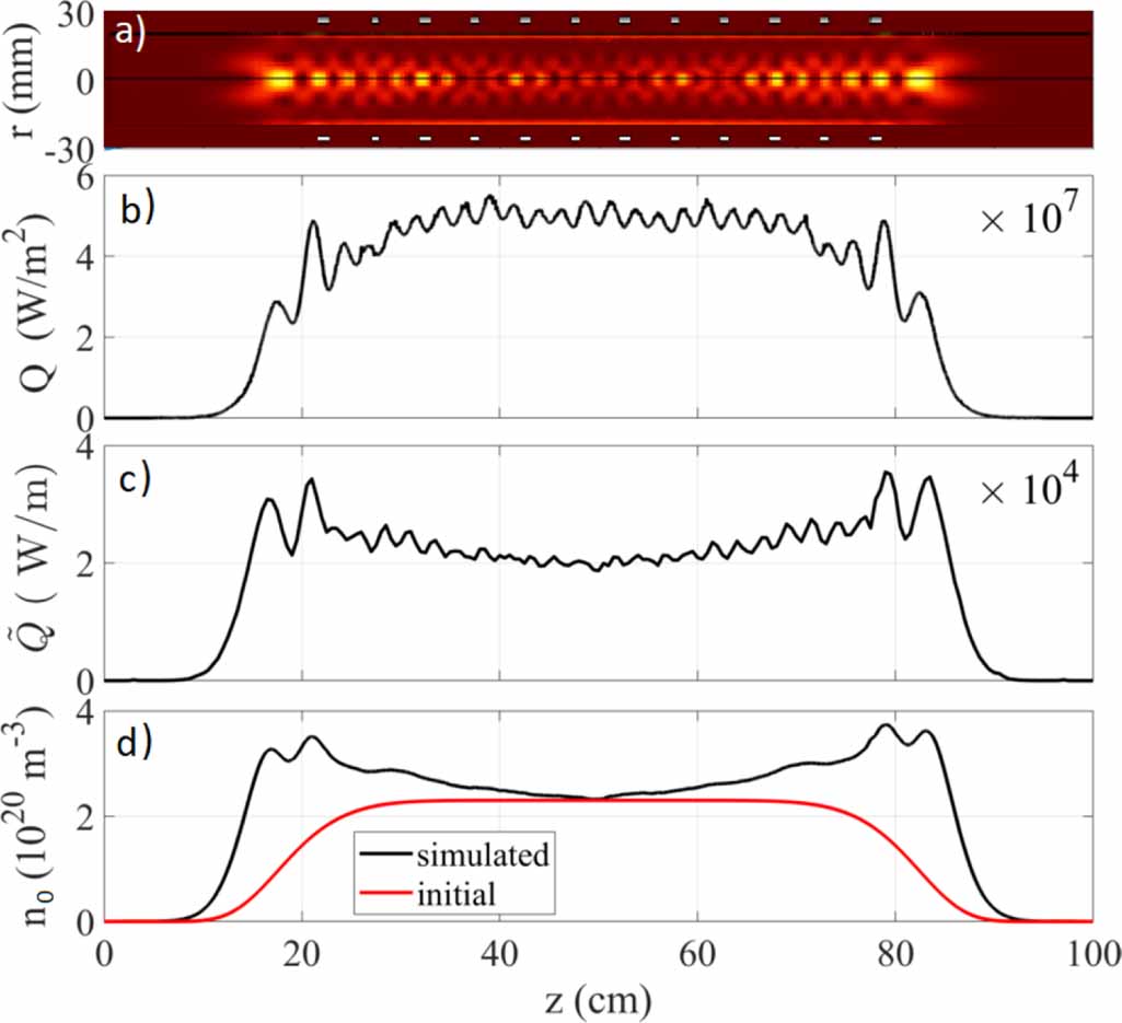
The most stringent requirement for the AWAKE accelerator plasma source is the homogeneity of the axial density profile of 0.25%. We here explore the achievable density homogeneity within the limits of the 1D simulation with an optimized HPS setup. We choose a target density of 2.3$\times 10^{-20}$ m⁻³ in order to be close to the experimental conditions that have been used to establish the simulation. A B-field of 0.1 T, constant along the entire simulation domain, is assumed. For these conditions, a single ring antenna excites a dominant mode with axial wavelength of 5 cm. Therefore, an antenna was placed every 5 cm along the ideal quartz tube. The overall 12 antennas are powered with 25 kW in total (2.1 kW/antenna) and the argon pressure is set to 8 Pa. Figure 13(a) shows the 2D deposited power map. An axial line-out at the center (figure 13(b)) illustrates a flat power deposition region in the central 0.5 m with an oscillation of 25 mm period and 10% amplitude in comparison to the average value. Integration over the radial variable (figure 13(c)) reduces the amplitude of the oscillations but introduces an over-all gradient resulting in a slightly lower power deposition in the center of the system. Figure 13(d) shows the resulting electron density from the PPM (black line), compared to the original density profile utilized to calculate the power deposition (red line). The mobility of the particles smooths out the oscillations but the density gradient seen in figure 13(c) is still present. We achieve here an axial variation of the electron density of $\pm 10\%$ over the central 0.5 m of the HPS. This is a significant improvement over the $\pm 50\%$ density variation predicted for the present experiment (3 antennas, strongly varying axial B-field), but still far from the 0.25% required for AWAKE experiments.

Zoom In Zoom Out Reset image size

However, it is plausible that the actual density profile in the presented case is closer to the on-axis power profile (figure 13(b)) than to the radially integrated case (figure 13(c)). This highlights the need to develop a 2D-model that can take into account the full map of the power deposited into the plasma. Furthermore, we find that the power deposition pattern is dominated by the near field of the antennas and that a variation of the initial electron density or the exact antenna spacing can result in strongly varying interference patterns. However, these fluctuations have only a minor influence on the resulting n_e profile, so that an even closer spacing of the antennas is not resulting in a more homogeneous plasma density. The simulations suggest that a setup with an antenna spacing around 5 cm could be suitable to achieve a relatively homogeneous n_e profile in a range of electron density amplitudes. The density tuning could be achieved by the power and DC magnetic field applied to the system.