Fastcc: Fast Color Corrections for Broadband Radio Telescope Data

Cosmic Microwave Background (CMB) observations require telescopes using high sensitivity receivers with wide bandwidths that are a large fraction of the observing frequency. For example, the 28.4 GHz channel of the Planck satellite was sensitive to photons at frequencies between ∼24 and 34 GHz (see Figure 1), a fractional bandwidth (i.e., Δν/ν) of ∼35%. With such high fractional bandwidths, the measured flux density of an astronomical source depends on the convolution of the observing spectral bandpass with the source spectrum. For example, a bandpass that is most sensitive at low frequencies will result in an increase in the measured flux density of a steep spectrum radio source compared to a flatter spectrum source. Color corrections avoid these effects by correcting the flux density to that which a monochromatic receiver operating at a reference frequency ν₀ would have measured.

Zoom In Zoom Out Reset image size

The color correction thus depends on the spectral index of the source, and if the value for this changes (e.g., while fitting a model with multiple spectral components, or when adding new observations), then the color correction also changes. For this reason, raw flux densities are published without color corrections, but color corrections are applied for any scientific analysis and for the inclusion of data in data visualization and subsequent analysis.

The fastcc and interpcc codes provide fast color corrections for CMB data sets, particularly in MCMC fitting techniques.

We follow and expand on the formalism from Planck Collaboration (2016). When the source spectrum is described by a power-law, S ∝ ν^α , the color correction is the ratio of integrals over frequency ν, with the numerator integrating over the bandpass g(ν) (if measured in temperature units) and the spectrum the data is calibrated to, δ, and the denominator integrating over the combination of the bandpass and the source spectrum with spectral index α, as

$$\begin{eqnarray}&&C({\nu }_{0},\alpha )=\displaystyle \frac{\int g(\nu ){\left(\nu /{\nu }_{0}\right)}^{\delta -2}\,d\nu }{\int g(\nu ){\left(\nu /{\nu }_{0}\right)}^{\alpha -2}\,d\nu },\end{eqnarray} \tag{ 1 }$$

where ν₀ is the reference frequency. If the instrument bandpass has been measured in intensity units, τ(ν), this becomes:

$$\begin{eqnarray}&&C({\nu }_{0},\alpha )=\displaystyle \frac{\int \tau (\nu ){\left(\nu /{\nu }_{0}\right)}^{\delta }\,d\nu }{\int \tau (\nu ){\left(\nu /{\nu }_{0}\right)}^{\alpha }\,d\nu }.\end{eqnarray} \tag{ 2 }$$

For instruments calibrated in CMB thermodynamic units, this becomes:

$$\begin{eqnarray}&&C({\nu }_{0},\alpha )=\displaystyle \frac{\int g(\nu ){\eta }_{{\rm{\Delta }}T}(\nu )/{\eta }_{{\rm{\Delta }}T}({\nu }_{0})\,d\nu }{\int g(\nu ){\left(\nu /{\nu }_{0}\right)}^{\alpha -2}\,d\nu },\end{eqnarray} \tag{ 3 }$$

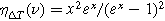where ${\eta }_{{\rm{\Delta }}T}{(\nu )={x}^{2}{e}^{x}/({e}^{x}-1)}^{2}$, with x = h ν/(k_B T_CMB) to adjust for the CMB spectrum in Rayleigh–Jeans temperature units, with Planck constant h, Boltzmann constant k_B, and CMB temperature T_CMB = 2.7255 K. However, the ratio of η_ΔT is usually small, only becoming important when ν₀ is far from the center of the bandpass.

The resulting color corrections are very smooth (see Figure 1, right), and can be fitted with a quadratic function:

$$\begin{eqnarray}&&C({\nu }_{0},\alpha )={c}_{0}+{c}_{1}\alpha +{c}_{2}{\alpha }^{2}.\end{eqnarray} \tag{ 4 }$$

The source flux density is then corrected as:

$$\begin{eqnarray}\begin{array}{rcl}{S}_{\mathrm{corr}}({\nu }_{0}) & = & {S}_{\mathrm{orig}}({\nu }_{0})C({\nu }_{0},\alpha )\\ & = & {S}_{\mathrm{orig}}({\nu }_{0})\times \left({c}_{0}+{c}_{1}\alpha +{c}_{2}{\alpha }^{2}\right).\end{array}\end{eqnarray} \tag{ 5 }$$

The color corrections for thermal dust spectra can be calculated using the same equations as for power laws, but changing the source spectrum for a graybody, with the dust temperature T_dust and spectral index β_dust as input parameters. For equations, see the fastcc explanatory supplement. A quadratic fit becomes increasingly different from the color corrections at extreme values. As such, we also include interpcc, which uses interpolation over a set of cached color correction values.

There are two equivalent approaches to color correction: either change the flux density of the source at a fixed reference frequency, or change the reference frequency for the observations. When characterizing multiple sources within a survey, the analysis is normally simpler if all sources are at the same frequency with corrected flux density. Alternatively, effective frequencies ν_eff, for which C(ν_eff, α) = 1, can be calculated from the color corrections (in thermodynamic units: convert to intensity at ν_eff) via:

$$\begin{eqnarray}&&{\nu }_{\mathrm{eff}}={\nu }_{0}C{\left({\nu }_{0},\alpha \right)}^{1/(\alpha -2)}.\end{eqnarray} \tag{ 6 }$$

The code takes input α for fastcc, or T_dust, and β_dust for interpcc, and returns the factor that the measured flux density must be multiplied to obtain the corrected flux density. We include both Python and IDL versions of fastcc, and interpcc in Python. Test/example scripts are also included for both fastcc and interpcc. The code is available at https://github.com/mpeel/fastcc and 10.5281/zenodo.7376510 , along with a more detailed explanatory supplement. An IDL version for Planck LFI only was released in the Planck Legacy Archive. ⁵ While no dependencies are required for fastcc, interpcc and the color correction calculations use Astropy (Astropy Collaboration et al. 2018), Numpy (Harris et al. 2020), and scipy (Virtanen et al. 2020).

The code now includes color corrections for Planck LFI (Planck Collaboration 2014a, 2014b, 2016) and HFI (Planck Collaboration 2014b), WMAP (Bennett et al. 2013), IRAS (IRAS 1988), DIRBE, ⁶ QUIJOTE MFI (Rubiño-Martín et al. 2022, MNRAS in press; Genova-Santos et al. 2022, in preparation), and C-BASS (King et al. 2014; Taylor et al. 2022, in preparation). Additional experiments can be added on request and provision of bandpasses.