


 t 19c, B-4000 Liège, Belgium

Abstract
We present JWST-MIRI Medium Resolution Spectrometer (MRS) spectra of the protoplanetary disk around the low-mass T Tauri star GW Lup from the MIRI mid-INfrared Disk Survey Guaranteed Time Observations program. Emission from 12CO2, 13CO2, H2O, HCN, C2H2, and OH is identified with 13CO2 being detected for the first time in a protoplanetary disk. We characterize the chemical and physical conditions in the inner few astronomical units of the GW Lup disk using these molecules as probes. The spectral resolution of JWST-MIRI MRS paired with high signal-to-noise data is essential to identify these species and determine their column densities and temperatures. The Q branches of these molecules, including those of hot bands, are particularly sensitive to temperature and column density. We find that the 12CO2 emission in the GW Lup disk is coming from optically thick emission at a temperature of ∼400 K. 13CO2 is optically thinner and based on a lower temperature of ∼325 K, and thus may be tracing deeper into the disk and/or a larger emitting radius than 12CO2. The derived  /
/ ratio is orders of magnitude higher than previously derived for GW Lup and other targets based on Spitzer-InfraRed-Spectrograph data. This high column density ratio may be due to an inner cavity with a radius in between the H2O and CO2 snowlines and/or an overall lower disk temperature. This paper demonstrates the unique ability of JWST to probe inner disk structures and chemistry through weak, previously unseen molecular features.
Export citation and abstract BibTeX RIS

Original content from this work may be used under the terms of the Creative Commons Attribution 4.0 licence. Any further distribution of this work must maintain attribution to the author(s) and the title of the work, journal citation and DOI.
1. Introduction
The inner 10 au of protoplanetary disks are regions of active chemistry, with high temperatures and densities and with the snowlines of H2O and CO2 controlling the gas composition (e.g., Pontoppidan et al. 2014; Walsh et al. 2015; Bosman et al. 2022). The chemistry in this region is expected to impact the atmospheric compositions of any exoplanets, the bulk of which are expected to form in this region (Dawson & Johnson 2018; Öberg & Bergin 2021; Mollière et al. 2022), which is difficult to probe with the Atacama Large Millimeter/submillimeter Array (ALMA).
Of the several species that emit from the inner ∼10 au of disks, CO2 is a particularly informative tracer of the physical and chemical conditions in this region. In the interstellar medium, ices are rich in CO2 (abundances of 10−5 with respect to the total gas density; de Graauw et al. 1996; Gibb et al. 2004; Bergin et al. 2005; Pontoppidan et al. 2008; Boogert et al. 2015). However, the CO2 abundance in disks, derived from both local thermodynamic equilibrium (LTE) slab models and full disk non-LTE modeling of Spitzer-InfraRed-Spectrograph (IRS) observations, is between 10−9 and 10−7 with respect to the total gas density, indicating reprocessing in the disk (Salyk et al. 2011; Pontoppidan & Blevins 2014; Bosman et al. 2017). Despite these lower disk abundances, Pontoppidan et al. (2010) found that CO2 was the second most common molecule detected in disks (20 disks) after water (25 disks) in a sample of 73 protoplanetary disks observed with Spitzer-IRS. In those sources, the CO2 Q branch at 14.9 μm was useful as a diagnostic of the gas temperature and abundance in their inner regions. Besides ice production, CO2 is also formed in the gas phase at moderate temperatures (100–200 K) through the reaction of CO + OH → CO2 + H. At higher temperatures, OH primarily reacts with H2 to form H2O. Thus, the CO2/H2O ratio is sensitive to the gas temperature.
Despite the usefulness of its typically bright Q branch, 12CO2 is thought to be largely optically thick in the regions of the disk where it is emitting (Bosman et al. 2017). Therefore, optically thinner lines and isotopologues are more useful in determining the column density of CO2, as well as the physical and chemical conditions in the disk. Moderate spectral resolution and high signal-to-noise observations are needed to detect the weaker optically thin lines and isotopologues, which was not possible with Spitzer. JWST-MIRI provides a new opportunity to study the Q branches of 12CO2 and 13CO2, and the ability to identify individual P- and R-branch lines for 12CO2.
We present JWST-MIRI observations of one of the CO2-bright sources identified in Spitzer observations: GW Lup (Pontoppidan et al. 2010; Salyk et al. 2011; Bosman et al. 2017). GW Lup (Sz 71) is an M1.5 star (Teff = 3630 K, L* = 0.33 L⊙, M* = 0.46 M⊙) in the Lupus I cloud at a distance of 155 pc (Alcalá et al. 2017; Andrews et al. 2018). This target was observed as part of the DSHARP survey (Andrews et al. 2018), which found a very narrow ring of continuum emission at a radius of 85 au in addition to a centrally peaked continuum (Dullemond et al. 2018). We redetect C2H2 and strong 12CO2 emission in this disk (Pontoppidan et al. 2010; Salyk et al. 2011; Banzatti et al. 2020) and additionally detect 13CO2, H2O, HCN, and OH for the first time in this source. We fit the 13.6–16.3 μm wavelength range of the MIRI spectrum with LTE slab models to constrain the column density and temperature for each species. We discuss our findings, in particular the detection of 13CO2, which is the first such detection in a protoplanetary disk, and the column density ratio of CO2 to H2O, which provides new insight into the inner disk structure.
2. Observations and Analysis
2.1. Observations and Data Reduction
GW Lup was observed with the Mid-InfraRed Instrument (MIRI; Rieke et al. 2015; Wells et al. 2015; Wright et al. 2015, Wright et al. 2023, I. Argyriou et al. 2023, in preparation) in the Medium Resolution Spectroscopy (MRS) mode on 2022 August 8. These observations are part of the MIRI mid-INfrared Disk Survey (MINDS) JWST Guaranteed Time Observations Program (PID: 1282, PI: T. Henning). Target acquisition was used so that a point-source fringe flat could be used in the data reduction. A four-point dither was performed in the positive direction. The total exposure time was 1 hr. All the JWST data used in this paper can be found in MAST doi:10.17909/aez2-za93.
The MIRI MRS observations were processed through all three reduction stages (Bushouse et al. 2022) using Pipeline version 1.8.4. The reference files were generated from the observation of the reference A-type star HD 163466. Additional details on the reference files used can be found in Gasman et al. (2023). A single dedicated point-source fringe flat and dedicated spectrophotometric calibration were used in the reduction process. We skip the outlier rejection step in Spec3, as this produces spurious results due to the undersampling of the point-spread function (PSF), causing undersampling artifacts (e.g., short-period oscillations at the beginning and end of each subband) in the extracted spectrum. Undersampling of the PSF and its artifacts will be discussed in an upcoming paper (D. R. Law et al. 2023, in preparation). Finally, the centroid of the PSF was found manually prior to the extraction of the spectra in each subband, which included aperture correction, with an aperture size of 2.5λ/D. The correction factors are the same as those presented in I. Argyriou et al. (2023, in preparation), which include the contribution of the PSF wings to the estimated background determined from an annulus around the source. The background emission from this annulus is subtracted and its value ranges from ∼0.001 Jy in Channel 1 to ∼0.1 Jy around 22 μm. The continuum emission is not extended in the 2D images; therefore, the disk is not resolved.
The final GW Lup spectrum through Channel 4A is presented in Figure 1. At longer wavelengths the flux calibration becomes increasingly uncertain, due to the low flux level at these wavelengths in the reference star used for calibration; therefore, we only show through Channel 4A. The ν2 = 1–0 12CO2 Q branch is the most prominent, but a large number of weaker lines are detected as well. A spurious, single-pixel spike at 18.8 μm has been removed. Below 7.5 μm, the Spitzer low-resolution spectrum of GW Lup has a ∼20% higher flux. However, above 7.5 μm, the flux of the JWST-MIRI spectrum is ∼15% higher than the Spitzer-IRS high- and low-resolution spectra of this target, but the overall shape is very similar (see Figure 5 in the Appendix). These offsets may be due to calibration issues and/or variability in this system. This will be investigated in a future work. In this work, we use the MIRI continuum-subtracted spectrum for analysis.

Figure 1. The JWST-MIRI MRS spectrum for GW Lup through Channel 4A. Several of the strongest emission features are labeled and insets show additional molecular features. The beginning and end of each subband has been trimmed to reduce spurious features due to the increased noise at the ends of the bands.
Download figure:
Standard image High-resolution image2.2. Slab Modeling Procedure
The MIRI spectrum is continuum subtracted in the 13–17 μm range by selecting regions with minimal line emission and using a cubic spline interpolation to determine the continuum level. This continuum is then subtracted from the observed spectra (see Appendix B and Figure 6 for more details).
We fit the 13–16.3 μm continuum-subtracted spectrum with LTE slab models. The line profile function is assumed to be Gaussian with an FWHM of ΔV = 4.7 km s−1 (σ = 2 km s−1) as is done in Salyk et al. (2011), which represents the line width for H2 at 700 K. This value does not have a large impact on the results and we adopt the value of Salyk et al. (2011) for consistency. The model takes into account the mutual shielding of adjacent lines for the same species. In particular, the total opacity is first computed on a fine wavelength grid by summing the contribution of all the lines before computing the emerging line intensity. These models allow us to reproduce the data with only three free parameters: the line-of-sight column density N, the gas temperature T, and the emitting area given by πR2 for a disk of emission with radius R. While we report the emitting area in terms of this emitting radius, the emission could be coming from a ring with an area equivalent to πR2. We include emission from C2H2, HCN, H2O, 12CO2, 13CO2, and OH. The 12CO2, 13CO2, C2H2, and HCN line transitions are derived from the HITRAN database (Gordon et al. 2022). All the lines within 4–30 μm range are selected and are converted into LAMDA format (van der Tak et al. 2020) for compatibility with our slab model. The partition sums for these molecules are retrieved from the TIPS_2021_PYTHON package provided by the database. 24 The OH spectroscopy stems from Tabone et al. (2021) who used data from Yousefi & Bernath (2018) and Brooke et al. (2015). We vary the emitting area, as described below, and compute a synthetic spectrum in Jy, assuming a distance to GW Lup of 155 pc. The model spectrum is then convolved to a resolving power of 2500 for Channel 3 where the emission features are present (Labiano et al. 2021). Finally, the convolved model spectrum is resampled to have the same wavelength grid as the observed spectrum.
For each molecule, a grid of models was run with N from 1014 to 1022 cm−2, in steps of 0.166 in log10-space, and T from 100 to 1500 K, in steps of 25 K. The emitting area is varied by ranging the radius from 0.01 to 10 au in steps of 0.03 in log10-space. The best-fit N and T are determined using a χ2 fit (see Appendix C and Figure 7 for more details) between the continuum-subtracted data and the convolved and resampled model spectrum. For each N and T, the best-fit emitting area is determined by minimizing the χ2. The χ2 fit is done in spectral windows that are selected to minimize the contribution of emission from other species while still containing features that help to constrain the fits (e.g., optically thin lines and line peaks that are sensitive to temperature). This is done in an iterative approach to further reduce contamination from other species. The best-fit model is found for H2O first. This model is then subtracted from the observed, continuum-subtracted spectrum. We then fit HCN, subtract that model, and continue that procedure for C2H2, 12CO2, 13CO2, and then the final fit is done for OH. This is illustrated, with the spectral windows used for the χ2 determinations, in Figure 8 in Appendix C. After the initial best-fit models are found, this process is repeated for each molecule, after subtracting the best-fit models for all other species. For instance, the best-fit models for HCN, C2H2, 12CO2, 13CO2, and OH are subtracted from the observed spectra before the best-fit H2O model is found again (Figure 9). We repeat this process a third time, after which we see no further improvements in the residuals. The χ2 maps are shown in Appendix C (Figure 7).
3. Results
The best-fit model is presented in Figure 2 together with the continuum-subtracted spectrum in the 13.6–16.3 μm range. The best-fit model parameters are given in Table 1. The χ2 maps show that at low column densities (below ∼1017–1018 cm−2, depending on the molecule, see Figure 7), in the optically thin regime, the column density and emitting radius are completely degenerate (e.g., Salyk et al. 2011). In the optically thick regime, the emitting radius can more accurately be determined, although there is still a degeneracy between temperature and column density. Typical uncertainties can be read from the χ2 maps where the degeneracies are also evident. The degeneracy between our three free parameters is reduced by fitting a combination of optically thick and thin lines. For optically thin emission, the total number of molecules  = π N R2 is well determined and is included in Table 1. In GW Lup, we find that the emission of all species is optically thick, or at least on the border between optically thick and optically thin; therefore, the number of molecules should be taken as a lower limit.

Figure 2. The 13–16.3 μm wavelength range of the GW Lup spectrum, with the JWST-MIRI data (black) compared to a model (red) composed of emission from C2H2 (yellow), HCN (orange), H2O (blue), 12CO2 (green), 13CO2 (purple), and OH (pink). The inset shows a zoom-in of the 13CO2 feature.
Download figure:
Standard image High-resolution imageTable 1. Best-fit Model Parameters
| Species | N | T | R |
 a
a
|
|---|---|---|---|---|
| (cm−2) | (K) | (au) | (mol.) | |
| H2O | 3.2 × 10¹⁸ | 625 | 0.15 | 5 × 1043 |
| HCN | 4.6 × 10¹⁷ | 875 | 0.06 | 1.2 × 1042 |
| C2H2 | 4.6 × 10¹⁷ | 500 | 0.05 | 9.3 × 1041 |
| 12CO2 | 2.2 × 10¹⁸ | 400 | 0.11 | 1.7 × 1043 |
| 13CO2 | 1 × 10¹⁷ | 325 | 0.11 | 9.3 × 1041 |
| OH | 1 × 10¹⁸ | 1075 | 0.06 | 2.6 × 1042 |
Note.
a As the best-fit model parameters reported here are either totally in the optically thick regime or on the border between optically thick and thin, the total molecule number should be taken as a lower limit.Download table as: ASCIITypeset image
3.1. 12CO2 and 13CO2
Our best-fitting 12CO2 model has N = 2.2 × 1018 cm−2, a temperature of 400 K, and an emitting radius of 0.11 au. 12CO2 is well constrained to a temperature below ∼700 K, with the shape of the main Q branch being particularly constraining for the temperature. Using similar models and a similar technique on Spitzer-IRS data, Salyk et al. (2011) fit the fundamental 12CO2 Q branch at 14.9 μm and find a temperature of 750 K, a column density of 1.6 × 1015 cm−2, and an emitting radius of 1.01 au. While this optically thin model from Salyk et al. (2011) reproduces the main 14.9 μm Q branch, it does not reproduce the 12CO2 hot-band Q branches at 13.9 and 16.2 μm (1000–0110) as well as the optically thick model does (Figure 3). An example of the effect of changing the temperature by ± 100 K and column density by ± 0.5 dex on the 12CO2 model is shown in the Appendix in Figure 10.

Figure 3. Zoom-ins of the 15 μm wavelength range of GW Lup, with the JWST-MIRI data (black) compared to a model (red) composed of emission from 12CO2 (green) and 13CO2 (purple). The continuum and the best-fit models of C2H2, HCN, H2O, and OH shown in Figure 2, have been subtracted from the GW Lup spectrum. The top row shows the best optically thick fit from Figure 2, while the bottom row shows the optically thin 12CO2 fit from Salyk et al. (2011). The optically thick model reproduces the 12CO2 hot-band Q branches at 13.9 and 16.2 μm better than the optically thin model. In the optically thin case, a 12CO2/13CO2 ratio of 68 is not able to reproduce the 13CO2 Q branch at 15.4 μm.
Download figure:
Standard image High-resolution imageFor 13CO2, models from both the optically thick and optically thin regimes reproduce the feature well. With respect to 12CO2, the standard 12CO2/13CO2 abundance ratio of 68 from the local interstellar medium (Wilson & Rood 1994; Milam et al. 2005) is within the allowable range. The 13CO2 temperature is lower than that of 12CO2, with the best-fit temperature of 325 K. This indicates that the optically thinner 13CO2 is tracing deeper layers into the disk or larger radii (e.g., in a thin annulus farther out than the 12CO2, but with the same emitting area). The combination of 13CO2 and the P(23) line of 12CO2, reproduces the feature at 15.42 μm.
3.2. H2O
We include emission from both para- and ortho-water, assuming ortho/para = 3 (e.g., van Dishoeck et al. 2021 and references therein). Many H2O lines are present in the 13–17 μm region in the GW Lup spectra; however, they are weaker than the main CO2 Q branch and were not seen previously by Spitzer. An LTE slab model with a temperature of 625 K, a column density of 3.2 × 1018 cm−2, and an emitting radius of 0.15 au reproduces the lines in this region. This similar H2O column density compared to CO2 is in contrast to the much lower CO2/H2O ratios found in the large T Tauri Spitzer sample by Salyk et al. (2011), which is discussed in Section 4.
3.3. Other Species
For C2H2 and HCN (including the 0200–0110 HCN hot-band Q branch at 14.3 μm), the fits point to temperatures of ∼500 K and ∼875 K, respectively; however, this is quite unconstrained for C2H2, in particular. This high HCN temperature is needed to reproduce the ratio of line peaks in the main Q branch. The column densities for C2H2 and HCN are both on the border between being optically thick and optically thin. The emitting area for C2H2 and HCN is chosen from the best-fit model, but it is not well constrained. The OH emission is weak in the GW Lup spectrum, leading to quite unconstrained parameters; however, it is clear that the temperature is high (≳1000 K). OH levels are likely out of thermal equilibrium with an excitation temperature set by nonthermal processes such as prompt emission (Carr & Najita 2014; Tabone et al. 2021) or chemical pumping (Liu et al. 2000).
4. Discussion
As CO2 and H2O are two of the main oxygen carriers in protoplanetary disks, the relative abundances of these species is informative. While H2O emission is present in the MIRI MRS spectrum of GW Lup, it is relatively weak compared to CO2 with an  /
/ ratio of ∼0.7. It should be stressed that column density ratios should not be equated with abundance ratios since the emission of different molecules (or even of different bands of the same molecule) may originate from different regions or layers of the disk (Bruderer et al. 2015; Woitke et al. 2018). Moreover, the emission seen at mid-infrared wavelengths only probes the upper layers of the disk above the τmid−IR = 1 contour where the dust continuum becomes optically thick. To infer local abundances and their ratios, retrieval methods such as used in Mandell et al. (2012) or full forward thermochemical models using a physical structure tailored to the GW Lup disk are needed. Such models are beyond the scope of this paper. However, given the relatively small difference in emitting radii between CO2 and H2O, it is still informative to put the column density ratio into perspective.
The large T Tauri Spitzer sample of Salyk et al. (2011) find a median  /
/ ratio of 5 × 10⁻⁴. However, the column density ratios from Salyk et al. (2011) are largely derived from the low column density and high temperature (optically thin) regime that we exclude using the weaker hot-band 12CO2
Q branches at 13.9 and 16.2 μm. If the best-fitting radii found for H2O and CO2 of 0.15 and 0.11 au, respectively, correspond to the actual emitting radius (i.e., not coming from a thin annulus at larger radii with the same emitting area), then we note that these radii are smaller than the estimated midplane snowline of H2O, which is at ∼0.3–0.4 au for the stellar mass of GW Lup (Mulders et al. 2015). At high temperatures greater than ∼250 K, OH will react with H2 to form H2O (Glassgold et al. 2009). Why, then, is CO2 so abundant relative to H2O at these temperatures and locations in this disk? We present three scenarios.
ratio of 5 × 10⁻⁴. However, the column density ratios from Salyk et al. (2011) are largely derived from the low column density and high temperature (optically thin) regime that we exclude using the weaker hot-band 12CO2
Q branches at 13.9 and 16.2 μm. If the best-fitting radii found for H2O and CO2 of 0.15 and 0.11 au, respectively, correspond to the actual emitting radius (i.e., not coming from a thin annulus at larger radii with the same emitting area), then we note that these radii are smaller than the estimated midplane snowline of H2O, which is at ∼0.3–0.4 au for the stellar mass of GW Lup (Mulders et al. 2015). At high temperatures greater than ∼250 K, OH will react with H2 to form H2O (Glassgold et al. 2009). Why, then, is CO2 so abundant relative to H2O at these temperatures and locations in this disk? We present three scenarios.
- 1.Temperature structure. The temperature structure of the disk, which is largely controlled by the stellar luminosity, has a large impact on the inner disk CO2 and H2O abundances and on their molecular emission (e.g., Walsh et al. 2015; Woitke et al. 2018; Anderson et al. 2021). Models and observations have shown that the inner disks around low-mass stars are richer in carbon-bearing species in the disk atmosphere than those around higher-mass stars (e.g., Pascucci et al. 2013; Walsh et al. 2015). GW Lup, with a stellar mass of 0.46 M⊙, may be a borderline case where the C/O in the infrared emitting region is moderately high, but not so high that C2H2 is booming. Additionally, it is clear that H2O is not so abundant in the upper layers that self-shielding is taking place, since 13CO2 is detected, indicating a deep layer of CO2. Bosman et al. (2022) show that this occurs if the vertical H2O column density remains low enough that water self-shielding is suppressed, producing more OH which is needed for additional CO2 formation. There is always some small amount of H2O in the disk atmosphere that is being dissociated by UV photons from the star, decreasing the water abundance. This may be contributing to the relatively weak H2O emission as some OH emission is detected. In the cooler disks around M-type stars, some of the oxygen may also be driven into the unobservable O2 rather than H2O, making the atmosphere appear to be carbon rich even though the C/O ratio is solar (Walsh et al. 2015). The moderately low luminosity of GW Lup may contribute to the the higher
 / determined here; however, GW Lup is not so low-mass that this is likely the sole explanation. Future observations of additional targets, will help to demonstrate the impact of temperature structure on the derived column densities.
 - 2.Pebble drift. If dust grains coated in CO2-rich ices are drifting inward from the outer disk without any traps halting the drift, the inner disk will be enriched in oxygen (Banzatti et al. 2020). However, if ice enrichment is taking place both CO2 and H2O should be enriched at a ratio of 0.2–0.3 (Boogert et al. 2015), but only if the ices are transported vertically and there is no chemical reset. There may still be additional H2O and CO2 hidden below the dust τ15μm = 1 line. Bosman et al. (2017) compare the flux of the 13CO2 Q-branch at 15.42 μm to the neighboring 12CO2 P(25) line at 15.45 μm, and show that this ratio is sensitive to enhancements of CO2 at its snowline. In GW Lup, the P(25) line is stronger than the P(23) line, indicative of a contribution from the 1110–1000 hot-band Q branch of 12CO2 that is only present at high temperatures/column densities and was not seen in the models of Bosman et al. (2017). Therefore, the P(25) line is not a good representative of an individual P-branch line at these J levels. Instead, the P(27) line at 15.48 μm can be used. From the best-fit models, the peak of the 13CO2 Q-branch is at 6.5 mJy, compared to 4.7 mJy for the P(27) line. In the modeling setup of Bosman et al. (2017), this 13CO2/P(27) line ratio of 1.4 points to a low outer (10−8 with respect to the total gas density) and high inner (10−6) disk CO2 abundance. While this is intriguing, further modeling efforts, such as the full 2D physical-chemical models used by Bosman et al. (2017), are needed to realistically compare the inner and outer disk CO2 distribution for GW Lup specifically.
- 3.Inner cavity and/or dust trap. If there is an inner gas and dust cavity in the disk that extends to between the H2O and CO2 snowlines (estimated at ∼0.4 and >1 au, respectively), the H2O will be suppressed but the CO2 will still be abundant in the gas phase. The models of T Tauri disks from Walsh et al. (2015) and Anderson et al. (2021) show that the column densities of H2O dominate over those of CO2 in the inner 1 au. A cavity or gap may be present in GW Lup, which would remove abundant H2O and result in the relatively strong CO2 lines and relatively weak H2O lines observed in the GW Lup disk. In this case, the H2O will only be present in the uppermost layers of the disk atmosphere or at the heated edge of the cavity/gap where the icy grains are warm enough to sublimate water ice and/or where any free volatile oxygen is driven into H2O. Anderson et al. (2021) find that the H2O flux decreases substantially if an inner gas cavity is present, while the CO2 flux is less affected due to having more contribution from emission at larger radii, although as they note, the fluxes may not accurately reflect the column densities and abundances. If there is a dust trap between the snowlines, either created by the same mechanism opening the cavity or by other means, water ice-rich grains could be trapped beyond the H2O snowline, keeping H2O from sublimating but allowing for the sublimation and enrichment of CO2. Such a small cavity cannot be seen in the ALMA data, even with the high resolution of the DSHARP data. A small cavity in the dust could be traced in the dust continuum with near-infrared interferometry, whereas a gas cavity could be traced using high-spectral-resolution spectroscopy, for instance, of the CO rovibrational lines at 4.7 μm (e.g., Brown et al. 2013; Banzatti et al. 2022). None of these data exist yet for the GW Lup disk.


As more sources are observed with JWST-MIRI, these scenarios can be explored further. For instance, looking for trends of the CO2 versus H2O as a function of stellar luminosity and outer disk dust radius will be very informative in distinguishing between the importance of temperature structure versus pebble drift, as was done with Spitzer data. In the meantime, GW Lup can be put into context with other sources based on the Spitzer fluxes. Banzatti et al. (2020) (re)determined molecular line fluxes for H2O, HCN, C2H2, and CO2 for the Spitzer sample. While GW Lup has a relatively high Q-branch CO2 flux and relatively low 17 μm H2O flux compared to other disks, it is not a complete outlier (converted to line luminosities for comparison; Figure 4). Several disks in the Spitzer survey analyzed by Pontoppidan et al. (2010), Salyk et al. (2011), and Banzatti et al. (2020) also show high CO2 fluxes and low water fluxes, including DN Tau, IM Lup, MY Lup, and CX Tau (Figure 4). With the sensitivity and resolution of MIRI, there are likely to be other disks that will show 13CO2 emission, which will allow us to derive strong constraints on the CO2 column density and  /
/ ratio in these disks.

Figure 4. The Spitzer CO2 Q branch vs. 17 μm H2O fluxes in the sample studied in Banzatti et al. (2020). Downward-facing triangles are those with CO2 not detected above 3σ, leftward-facing triangles are those with H2O not detected above 3σ, and open points are those with neither detected above 3σ. Blue points are stars with stellar masses between 0.1 and 0.5 M⊙, to be comparable to GW Lup (red), which has a stellar mass of 0.46 M⊙. We show the luminosities determined from Spitzer and JWST for GW Lup.
Download figure:
Standard image High-resolution image5. Summary and Conclusions
- 1.We identify 12CO2, 13CO2, H2O, HCN, C2H2, and OH in the JWST-MIRI spectrum of GW Lup. Using LTE slab models, we reproduce the 13.6–16.3 μm spectrum. H2O, HCN, 13CO2, and OH are detected for the first time in this disk, as the features had line/continuum ratios that were too low to be detectable at the spectral resolution of Spitzer-IRS.
- 2.The gas-phase 13CO2 detection is the first in a protoplanetary disk. This detection points to a high CO2 abundance deep into the disk, with a 12CO2 column density of 2.2 × 1018 cm−2, temperature of 400 K, and an emitting radius of 0.11 au. For 13CO2, the best-fit model has a column density of 1 × 1017 cm−2, temperature of 325 K, and an emitting radius of 0.11 au.
- 3.The column density ratio of CO2 to H2O, derived from LTE slab models (/0.7) that fit simultaneously the 12CO2 hot bands, is over 2 orders of magnitude higher than what has previously been found in typical T Tauri disks. This may indicate an inner cavity with a radius in between the H2O and CO2 midplane snowlines and/or an overall lower disk temperature.
- 4.While GW Lup has a high CO2 flux relative to H2O, as seen with Spitzer, it is not completely an outlier, suggesting that other disks, such as those around MY Lup, IM Lup, DN Tau, and CX Tau are good candidates for the detection of 13CO2.


Taken together, this study demonstrates that JWST-MIRI MRS has the ability to provide new and unique constraints on inner disk physical and chemical structures.
We thank the referee for thoughtful, constructive comments that improved the manuscript. The following National and International Funding Agencies funded and supported the MIRI development: NASA; ESA; Belgian Science Policy Office (BELSPO); Centre Nationale dEtudes Spatiales (CNES); Danish National Space Centre; Deutsches Zentrum fur Luft-und Raumfahrt (DLR); Enterprise Ireland; Ministerio De Economía y Competividad; Netherlands Research School for Astronomy (NOVA); Netherlands Organisation for Scientific Research (NWO); Science and Technology Facilities Council; Swiss Space Office; Swedish National Space Agency; and UK Space Agency.
E.v.D. acknowledges support from the ERC grant 101019751 MOLDISK and the Danish National Research Foundation through the Center of Excellence "InterCat" (DNRF150). B.T. is a Laureate of the Paris Region fellowship program (which is supported by the Ile-de-France Region) and has received funding under the Marie Sklodowska-Curie grant agreement No. 945298. D.G. would like to thank the Research Foundation Flanders for co-financing the present research (grant No. V435622N). T.H. and K.S. acknowledge support from the ERC Advanced Grant Origins 83 24 28. I.K., A.M.A., and E.v.D. acknowledge support from grant TOP-1614.001.751 from the Dutch Research Council (NWO). I.K. and J.K. acknowledge funding from H2020-MSCA-ITN-2019, grant No. 860470 (CHAMELEON). G.B. thanks the Deutsche Forschungsgemeinschaft (DFG) - grant 138 325594231, FOR 2634/2. O.A. and V.C. acknowledge funding from the Belgian F.R.S.-FNRS. I.A. and D.G. thank the European Space Agency (ESA) and the Belgian Federal Science Policy Office (BELSPO) for their support in the framework of the PRODEX Programme. D.B. has been funded by Spanish MCIN/AEI/10.13039/501100011033 grants PID2019-107061GB-C61 and No. MDM-2017-0737. A.C.G. has been supported by PRIN-INAF MAIN-STREAM 2017 and from PRIN-INAF 2019 (STRADE). T.P.R. acknowledges support from ERC grant 743029 EASY. D.R.L. acknowledges support from Science Foundation Ireland (grant No. 21/PATH-S/9339). L.C. acknowledges support by grant PIB2021-127718NB-I00, from the Spanish Ministry of Science and Innovation/State Agency of Research MCIN/AEI/10.13039/501100011033.
Appendix A: Comparison with Spitzer-IRS
The comparison between the MIRI MRS data and the Spitzer-IRS data for GW Lup is shown in Figure 5. A spurious, single-pixel spike at 18.8 μm has been removed from the MIRI spectrum, as in Figure 1.

Figure 5. The JWST-MIRI MRS spectrum for GW Lup is shown with the subbands in different colors. The Spitzer-IRS high-resolution (HR) and low-resolution (LR) data are shown for comparison.
Download figure:
Standard image High-resolution imageAppendix B: Continuum Subtraction
The continuum is determined using a cubic spline interpolation (scipy.interpolate.interp1d) between selected regions with minimal line emission in the spectrum (Figure 6). Because the molecular emission is so rich in this wavelength region, the continuum points are selected to lie between emission features, which we confirm with our best-fit models (bottom panel). Due to the high signal-to-noise of the data and the fact that molecular features are not expected to produce an underlying continuum level at the column densities determined for this source, regions of low emission can be taken as the continuum level.

Figure 6. Top: The 13–16.3 μm wavelength range of our JWST-MIRI MRS data of GW Lup (black). The continuum points that we select are shown as the red points and the interpolated continuum is shown as the red line. Middle: The continuum-subtracted spectrum. Bottom: The best-fit models, as in Figure 2, showing the continuum points relative to the molecular features.
Download figure:
Standard image High-resolution imageAppendix C: χ2 Procedure and Maps
The reduced χ2 maps for H2O, HCN, C2H2, 12CO2, 13CO2, and OH are shown in Figure 7. The reduced χ2 is determined using the following formula:

where N is the number of resolution elements in the spectral windows that the fit is done over and σ is the standard deviation in a region with minimal line emission from 15.90 to 15.94 μm (Figure 8). As the emitting radius is just a scaling factor, the degrees of freedom is only 2 for the column density and temperature. The contours in the reduced χ2 shown in Figure 7 are the 1σ, 2σ, and 3σ levels determined as  + 2.3,
  + 6.2, and
  + 11.8, respectively (see Press et al. 1992 and Table 1 and Equation (6) of Avni 1976). Any contribution from other species in this line-rich region of the spectrum increases the overall χ2 value, although the spectral windows are selected to minimize this contribution. The procedure is iterative, as described in Section 2.2, to reduce the influence of overlapping molecular features on the best-fit parameters for a given species. The best-fit models are shown in Figure 9, along with the final noise level of 0.44 mJy. Figure 10 shows the effects of changing temperature and column density on the CO2 model as an example.

Figure 7. The χ2 maps for H2O, HCN, C2H2, 12CO2, 13CO2, and OH (from top to bottom). The color scale shows  . The red, orange, and yellow contours correspond to the 1σ, 2σ, and 3σ levels. The white contours show the emitting radii in astronomical units, as given by the labels. The best-fit model is marked as the black plus. The best-fit model corresponds to
  /χ2 = 1. These maps correspond to the χ2 and uncertainties after the third round in the iterative fitting procedure. The blue curve in the 12CO2 plot is the best-fitting emitting radius for H2O for comparison.
Download figure:
Standard image High-resolution image
Figure 8. The best-fit model procedure is shown here. The top panel shows the best-fit H2O model (blue) overlaid on the continuum-subtracted JWST-MIRI spectrum. In the second panel, the black spectrum is the observed spectrum after subtracting the H2O model from the first panel. The best-fit HCN model is found using this as the input spectrum. This process continues down the panels. The spectral windows used for each species fit are shown as the horizontal bars, with the given starting and ending points. A region with minimal line emission from 15.90 to 15.94 μm is chosen to determine the noise level (top panel). This region, before subtracting the models has a standard deviation of 0.76 mJy; however, some low-level molecular emission is still present.
Download figure:
Standard image High-resolution image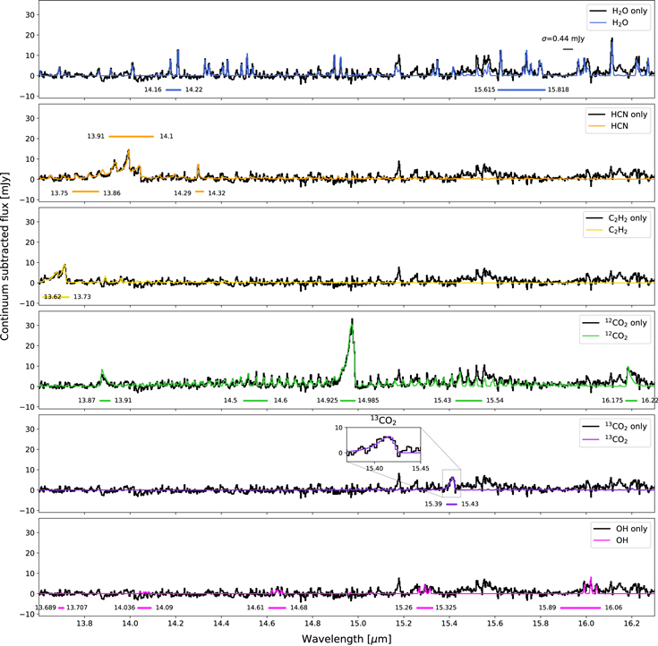
Figure 9. The same as Figure 8, but now showing the final best fits after the iterative process. The spectra shown in black are the observed data after subtracting the best-fit models from the previous iterations for all molecules except that being fitted; these spectra are what is used in determining the best-fit for the species in each panel. The noise level is decreased from Figure 8 because the excess emission, mostly from 12CO2 in this region has been removed.
Download figure:
Standard image High-resolution image
Figure 10. The 12CO2-only data, as in Figure 9, with models showing the impact of temperature (± 100 K; top) and column density (± 0.5 dex; bottom). The emitting area for the models has been chosen to best match the data. The best-fit model found for 12CO2, with a temperature of 400 K and a column density of 2.2 × 1018 cm−2, is shown in green. The temperature controls the width of the Q branches and the column density controls the position of the main Q-branch peak and the height of the hot-band peaks.
Download figure:
Standard image High-resolution image