


Abstract
We reassess the 65As(p,γ)66Se reaction rates based on a set of proton thresholds of 66Se, Sp(66Se), estimated from the experimental mirror nuclear masses, theoretical mirror displacement energies, and full pf-model space shell-model calculation. The self-consistent relativistic Hartree–Bogoliubov theory is employed to obtain the mirror displacement energies with much reduced uncertainty, and thus reducing the proton-threshold uncertainty up to 161 keV compared to the AME2020 evaluation. Using the simulation instantiated by the one-dimensional multi-zone hydrodynamic code, Kepler, which closely reproduces the observed GS 1826−24 clocked bursts, the present forward and reverse 65As(p,γ)66Se reaction rates based on a selected Sp(66Se) = 2.469 ± 0.054 MeV, and the latest 22Mg(α,p)25Al, 56Ni(p,γ)57Cu, 57Cu(p,γ)58Zn, 55Ni(p,γ)56Cu, and 64Ge(p,γ)65As reaction rates, we find that though the GeAs cycles are weakly established in the rapid-proton capture process path, the 65As(p,γ)66Se reaction still strongly characterizes the burst tail end due to the two-proton sequential capture on 64Ge, not found by the Cyburt et al. sensitivity study. The 65As(p,γ)66Se reaction influences the abundances of nuclei A = 64, 68, 72, 76, and 80 up to a factor of 1.4. The new Sp(66Se) and the inclusion of the updated 22Mg(α,p)25Al reaction rate increases the production of 12C up to a factor of 4.5, which is not observable and could be the main fuel for a superburst. The enhancement of the 12C mass fraction alleviates the discrepancy in explaining the origin of the superburst. The waiting point status of and two-proton sequential capture on 64Ge, the weak-cycle feature of GeAs at a region heavier than 64Ge, and the impact of other possible Sp(66Se) are also discussed.
Export citation and abstract BibTeX RIS

Original content from this work may be used under the terms of the Creative Commons Attribution 4.0 licence. Any further distribution of this work must maintain attribution to the author(s) and the title of the work, journal citation and DOI.
1. Introduction
During the accretion of stellar matter from a close companion by the neutron star in a low-mass X-ray binary, the accreted stellar matter, mainly comprising H and He fuses to heavier nuclei in steady-state burning (Schwarzschild & Härm 1965; Hansen & van Horn 1975) and a thermonuclear runaway is likely to occur in the accreted envelope of the neutron star. This causes the observed thermonuclear (Type I) X-ray bursts (XRBs; Woosley & Taam 1976; Maraschi & Cavaliere 1977; Joss 1977; Lamb & Lamb 1978; Bildsten 1998). The burst light curve, usually observed in X-rays, is the important observable indicating an episode of XRB, which can be either a series of XRBs or a single XRB, for instance, the XRBs recorded by the Rossi X-ray Timing Explorer (RXTE) Proportional Counter Array (Galloway et al. 2004, 2008, 2020). For a series of XRBs, we can further deduce the recurrence time between two XRBs, or the averaged recurrence time of a series of XRBs. The burst light-curve profile and (averaged) recurrence time can be studied via models best matching with observations to further understand the role of an important reaction, e.g., see Cyburt et al. (2016); Meisel (2018).
In recent years, the Type I clocked XRBs from the GS 1826−24 X-ray source (Makino 1988; Tanaka 1989; Ubertini et al. 1999) became the primary target of investigation due to its almost constant accretion rate and consistent light-curve profile (Heger et al. 2007; Paxton et al. 2015; Meisel 2018; Meisel et al. 2019; Dohi et al. 2020, 2021; Johnston et al. 2020). The other important feature of the GS 1826−24 clocked burster is the nuclear reaction flow during its XRB onsets. It can reach up to the SnSbTe cycles according to the models (Woosley et al. 2004) used by Cyburt et al. (2016) and Jacobs et al. (2018) to investigate the sensitivity of reactions. The region around SnSbTe cycles was found to be the endpoint of nucleosynthesis of an XRB (Schatz et al. 2001).
This state-of-the-art GS 1826−24 model was even recently advanced by the newly deduced 22Mg(α,p)25Al reaction rate to match with observation (Hu et al. 2021). As the abundances of synthesized isotopes are not observed, we remark here that using a set of high-fidelity XRB models capable of closely reproducing the observed burst light curves is important for us to diagnose the nuclear reaction flow and abundances of synthesized isotopes in the accreted envelope.
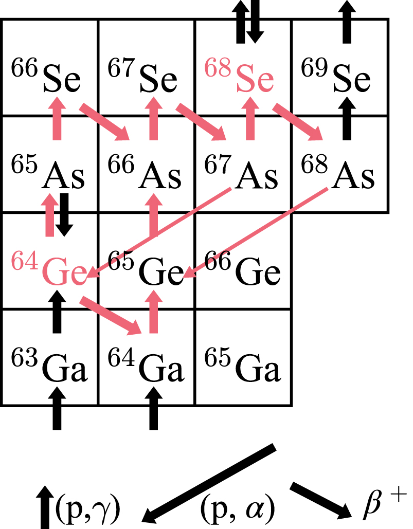
According to this GS 1826−24 model (Heger et al. 2007; Cyburt et al. 2016; Jacobs et al. 2018; Johnston et al. 2020; Hu et al. 2021; Lam et al. 2022), throughout the course of the XRBs of the GS 1826−24 clocked burster, the nuclear reaction flow has to break out from the ZnGa cycles to reach the GeAsSe region. The reaction flow inevitably goes through the 64Ge waiting point and also the GeAs cycles that might exist (Van Wormer et al. 1994) before surging through the region heavier than the Ge and Se isotopes where hydrogen is intensively burned. The GeAs cycles are supposedly weaker than the NiCu and ZnGa cycles due to the competition between the weak (p,α) and the strong (p,γ) reactions at As isotopes, see the weak GeAs I, II, and sub-II cycles presented in Figure 1. Thus, the establishment of the two-proton- (2p) sequential capture (hereafter 2p-capture) on 64Ge could be crucial to draw synthesized materials to follow the 64Ge(p,γ)65As(p,γ)66Se(β+ ν)66As(p,γ)67Se(β+ ν)67As(p,γ)68Se(β+ ν)68As(p,γ)69Se path for the strong rp-process of hydrogen (H)-burning that happens in nuclei heavier than Se isotopes.

Figure 1. The rapid-proton capture (rp-) process path passing through the weak GeAs cycles. Waiting points are shown in red. The GeAs cycles are displayed as red arrows. The GeAs I cycle consists of 64Ge(p,γ)65As(p,γ)66Se(β+ ν)66As(p,γ)67Se(β+ ν)67As(p,α)64Ge reactions (Van Wormer et al. 1994), and the GeAs II cycle involves a series of 65Ge(p,γ)66As(p,γ)67Se(β+ ν)67As(p,γ)68Se(β+ ν)68As(p,α)65Ge reactions. The other sub-GeAs II cycle, 64Ge(β+ ν)64Ga(p,γ)65Ge(p,γ)66As(p,γ)67Se(β+ ν)67As(p,α)64Ge, may also be established. The weak (p,α) reactions are represented by thinner arrows.
Download figure:
Standard image High-resolution imageRecently, the role of 64Ge as an important waiting point was questioned when the proton threshold of 65As was experimentally deduced, opening a 2p-capture channel (Tu et al. 2011); its significance of an important waiting point also becomes uncertain in a study using a one-zone XRB model with the 64Ge(p,γ)65As and 65As(p,γ)66Se reaction rates deduced from the evaluated 65As and 66Se proton thresholds (Tu et al. 2011; Audi et al. 2017) and the full p f-model space shell-model calculation (Lam et al. 2016). Moreover, Schatz (2006) and Schatz & Ong (2017) found that the 65As and 66Se masses contributed to the respective proton thresholds affect the (p,γ) reverse rate, and hence influence the modeled XRB light curves. We remark that the investigations of the role of 64Ge as an important waiting point and the impact of 65As and 66Se masses were, however, based on the computationally effective zero-dimensional one-zone XRB model (Schatz & Ong 2017) with extreme parameters, i.e., very high accretion rate and very low crustal heating, of which the abundance of synthesized nuclei is only provided for a single mass zone but not along the mass coordinate in the accreted envelope. A finer parameter range can be chosen to improve the capability of one-zone XRB models in estimating the influence of a particular reaction on XRB with agreement close to the one-dimensional multi-zone hydrodynamic XRB model (H. Schatz 2021, private communication). Notably, the hydrodynamic data generated from a more constrained one-dimensional multi-zone XRB model that is capable of reconciling theoretical light curves with observations could be beneficial for post-processing and one-zone models to obtain the nuclear energy generation (XRB flux) consistent with the input hydrodynamic snapshots and to assess the inventory of abundances and the reaction flow during the burst.
With the advantage of new and high intensity exotic proton-rich isotopes production and advances in experimental techniques of isochronous mass spectrometry in storage rings (Stadlmann et al. 2004; Zhang et al. 2018) and multi-reflection time-of-flight (MRTOF) mass spectrometers (Wolf et al. 2013; Dickel et al. 2015; Jesch et al. 2015; Rosenbusch et al. 2020), the 66Se proton threshold, Sp(66Se), could be more precisely determined to replace the Sp(66Se) = 2.010 ± 220 MeV predicted by AME2020 extrapolation (Kondev et al. 2021; AME2020). The extrapolation is based on the trend from the mass surface, which is weak in predicting proton-rich nuclear masses due to the shell effect originating from the respective shell structure or the configuration of the ground state (W. J. Huang 2021, private communication). Therefore, a set of forefront investigations on astrophysical impacts due to the forward and reverse 65As(p,γ)66Se reactions based on a set of Sp(66Se) with lower uncertainty than the one predicted by AME2020 and XRB models best matching with observation is highly desired.
In Section 2, we present the formalism obtaining the forward and reverse 65As(p,γ)66Se reaction rates, and discuss these newly deduced forward and reverse reaction rates. We then employ the one-dimensional multi-zone hydrodynamic Kepler code (Weaver et al. 1978; Woosley et al. 2004; Heger et al. 2007) to instantiate XRB simulations that produce a set of XRB episodes matched with the GS 1826−24 clocked burster with the newly deduced 65As(p,γ)66Se forward and reverse reaction rates. Other recently updated reaction rates, i.e., 55Ni(p,γ)56Cu (Valverde et al. 2019), 56Ni(p,γ)57Cu (Kahl et al. 2019), 57Cu(p,γ)58Zn (Lam et al. 2022), and 64Ge(p,γ)65As (Lam et al. 2016) around the historic 56Ni and 64Ge waiting points, and 22Mg(α,p)25Al (Hu et al. 2021) at the important 22Mg branch point are also taken into account. In Section 3, we study the influence of these 65As(p,γ)66Se forward and reverse rates, and also investigate the influence of the 2p-capture on 64Ge and GeAs cycles on XRB light curves, on the rp-process path during the thermonuclear runaway of the GS 1826−24 clocked XRBs, and on the nucleosyntheses in and evolution of the accreted envelope along the mass coordinate for nuclei of mass A = 59, ..., 68. The conclusions of this work are given in Section 4.
2. Reaction Rate Calculations
We deduce the Sp(66Se) value based on the experimental 66Ge mirror mass and theoretical Coulomb displacement energy (and the term should be replaced as mirror displacement energy (MDE) due to the important role of isospin non-conserving forces from nuclear origin Zuker et al. 2002). The MDE is obtained from the self-consistent relativistic Hartree–Bogoliubov (RHB) theory (Kucharek & Ring 1991; Meng & Ring 1996; Ring 1996; Pöschl et al. 1997). The MDE for a given pair of mirror nuclei is expressed as (Brown et al. 2000, 2002; Zuker et al. 2002)

where A is the nuclear mass number and I is the isospin, BE  and BE
  are the binding energies of the proton- and neutron-rich nuclei, respectively. We implement the explicit density-dependent meson-nucleon couplings (DD-ME2) effective interaction (Lalazissis et al. 2005) in RHB calculations to obtain the MDE(A,I) of I = 1/2, 1, 3/2, and 2, A = 41–75 mirror nuclei. In order to constrict the complicated problem of a cutoff at large energies inherent in the zero range pairing forces, a separable form of the finite range Gogny pairing interaction is adopted (Tian et al. 2009). To describe the nuclear structure in odd-N and/or odd-Z nuclei, we take into account the blocking effects of the unpaired nucleon(s). The ground state of a nucleus with an odd neutron and/or proton numbers is a one-quasiparticle state,
  , which is constructed based on the ground state of an even–even nucleus ∣Φ0〉, where β† is the single-nucleon creation operator and ib denotes the blocked quasiparticle state occupied by the unpaired nucleon(s). A detailed description of implementing the blocking effect is explained in Ring & Schuck (1980).
Table 1 and Figure 2 present the Sp(66Se) values estimated from two mean field approaches, i.e., Skyrme Hartree–Fock (SHF) and RHB. For the SHF framework with the SkXcsb parameters (Brown 1998; Brown et al. 2002, 2000; B. A. Brown 2021, private communication), the previously estimated Sp(66Se) with the AME2000 66Ge and 65Ge binding energies is listed in the first row of Table 1, whereas the presently recalculated Sp(66Se) values with the AME2020 66Ge and 65Ge binding energies (Kondev et al. 2021) (SHFi), or with the AME2020 66Ge, 65Ge, and SHF MDEA=65 (SHFii), are arranged in the second and third rows of Table 1, respectively. For the RHB framework with DD-ME2 effective interaction, we deduce the Sp(66Se) using (I) the spherical harmonic oscillator basis and the AME2020 66Ge binding energy and theoretical or experimental MDEA=65 (RHB Sphericali,ii; the fourth and fifth rows in Table 1), (II) the axially symmetric quadrupole deformation and the AME2020 66Ge binding energy and theoretical or experimental MDEA=65 (RHB Axiali,ii; the sixth and seventh rows in Table 1).

Figure 2. The estimated Sp(66Se) from the SHF with SkXcsb interaction and from the RHB with DD-ME2 interaction using spherical harmonic oscillator basis or axially symmetric quadrupole deformation. The averaged Sp(66Se) from the SHF and from the RHB are  (66Se) = 2.323 ± 0.241 MeV (green dashed line) and
  (66Se) = 2.426 ± 0.163 MeV (red dashed line with red uncertainty zone), respectively. See text and Table 1.
Download figure:
Standard image High-resolution imageTable 1. Mirror Displacement Energies and Binding Energies of A = 65 and 66, and Sp(66Se)
| MDEA=66 | BE(66Ge) | BE(66Se) a | MDEA=65 | BE(65Ge) | BE(65As) a | Sp(66Se) | |
|---|---|---|---|---|---|---|---|
| SHF (SkXcsb) b | |||||||
| Brown et al. (2002) | 21.340 (100) b | −569.293 (30) c | −547.953 (104) | 10.491 (100) b | −556.011 (100) c | −545.520 (100) | 2.433 (144) |
| SHFi (AME2020) | 21.340 (100) b | −569.279 (2) d | −547.939 (100) | 10.326 (80) d | −556.079 (2) d | −545.753 (80) d | 2.186 (128) |
| SHFii (AME2020) | 21.340 (100) b | −569.279 (2) d | −547.939 (100) | 10.491 (100) b | −556.079 (2) d | −545.588 (100) | 2.351 (144) |
| RHB (DD-ME2) e | |||||||
| Sphericali (AME2020) | 21.083 (62)
| −569.279 (2) d | −548.196 (62) | 10.326 (80) d | −556.079 (2) d | −545.753 (80) d | 2.443 (101) |
| Sphericalii (AME2020) | 21.083 (62)
| −569.279 (2) d | −548.196 (62) | 10.389 (33)
| −556.079 (2) d | −545.690 (33) | 2.507 (70) |
| Axiali (AME2020) | 21.242 (46)
| −569.279 (2) d | −548.037 (46) | 10.326 (80) d | −556.079 (2) d | −545.753 (80) d | 2.284 (92) |
| Axialii (AME2020) | 21.242 (46)
| −569.279 (2) d | −548.037 (46) | 10.510 (29)
| −556.079 (2) d | −545.568 (29) | 2.469 (54) |
Notes.
a Deduced from , see, Equation (1), except otherwise quoted from the experiment.
b
Skyrme Hartree–Fock calculations with SkXcsb parameters (B. A. Brown 2021, private communication; Brown et al. 2002, 2000; Brown 1998).
c
Quoted from AME2000, which is a preliminary data set of AME2003 (Audi et al. 2003).
d
Quoted from AME2020 (Kondev et al. 2021).
e
RHB (Kucharek & Ring 1991; Ring 1996; Meng & Ring 1996; Pöschl et al. 1997) calculations with DD-ME2 effective interaction (Lalazissis et al. 2005), using (I) spherical harmonic oscillator basis, (II) axially symmetric quadrupole deformation. The 62 keV and 46 keV uncertainties of MDEA=66 are from the root-mean-square (rms) deviation value of comparing the theoretical and experimental MDE(A,I) values for I = 1, A = 42–58 mirror nuclei. We apply the same procedure to quantify the 33 keV and 29 keV uncertainties for the MDEA=65 considering I = 1/2, A = 41–75 mirror nuclei. The uncertainties of BE(66Se), BE(65As), Sp(66Se) are from the combination of rms deviation and the respective experimental uncertainty.
, see, Equation (1), except otherwise quoted from the experiment.
b
Skyrme Hartree–Fock calculations with SkXcsb parameters (B. A. Brown 2021, private communication; Brown et al. 2002, 2000; Brown 1998).
c
Quoted from AME2000, which is a preliminary data set of AME2003 (Audi et al. 2003).
d
Quoted from AME2020 (Kondev et al. 2021).
e
RHB (Kucharek & Ring 1991; Ring 1996; Meng & Ring 1996; Pöschl et al. 1997) calculations with DD-ME2 effective interaction (Lalazissis et al. 2005), using (I) spherical harmonic oscillator basis, (II) axially symmetric quadrupole deformation. The 62 keV and 46 keV uncertainties of MDEA=66 are from the root-mean-square (rms) deviation value of comparing the theoretical and experimental MDE(A,I) values for I = 1, A = 42–58 mirror nuclei. We apply the same procedure to quantify the 33 keV and 29 keV uncertainties for the MDEA=65 considering I = 1/2, A = 41–75 mirror nuclei. The uncertainties of BE(66Se), BE(65As), Sp(66Se) are from the combination of rms deviation and the respective experimental uncertainty.Download table as: ASCIITypeset image
The region around nuclei A = 65 and 66 is subject to deformation as found by Hilaire & Girod (2007); however, the SHF calculations do not take deformation into account. This somehow causes the SHF MDEs to have a large rms deviation of around 100 keV. The Sp(66Se) uncertainties of the SHF calculations are larger than the RHB calculations, whereas the RHB Axiali,ii uncertainties are lower than the ones from RHB Sphericali,ii. The uncertainty (rms deviation) of MDEs from RHB Sphericali,ii suggests that refitting the SkXcsb parameters and revising the blocking effect for calculating even–odd and odd–odd nuclei are likely to reduce the SHF uncertainty to around 60 keV. Nevertheless, the deformation of nuclei is not considered in both SHF and RHB Sphericali,ii calculations. The RHB Axiali,ii that take into account deformation further alleviate the discrepancy between theoretical and experimental MDEs, and thus reducing the uncertainty of the deduced Sp(66Se) values. This is exhibited by comparing the RHB Axiali,ii MDEA=66 46 keV and MDEA=65 29 keV uncertainties with the 62 and 33 keV (RHB Sphericali,ii) and with the 100 keV (SHF) uncertainties, see Table 1 and Figure 2. In addition, the RHB with DD-ME2 calculations have an advantage in that the meson-nucleon effective interaction is explicitly constructed without additional extra terms as included in the SHF calculation via the SkXcsb terms, which have to be continually refitted with updated experiments.
For the RHB calculations, we find that the RHB MDEs coupled with highly precisely measured 66Ge and 65Ge binding energies yield a set of Sp(66Se) values with low uncertainties, i.e., 2.507 ± 0.070 and 2.469 ± 0.054 MeV (fifth and seventh rows in Table 1). This indicates that the 80 keV uncertainty of 65As binding energy is somehow large enough to influence the deduced Sp(66Se), see the fourth and sixth rows in Table 1 and Figure 2, suggesting a highly precisely measured 65As mass is demanded. Furthermore, we also find that consistently using the RHB MDEs and precisely measured 66Ge and 65Ge binding energies maintains the global description feature provided by the RHB framework to describe MDEs along the nuclear region with a symmetric neutron-proton number.
The Sp(66Se) of RHB listed in Table 1 is averaged to be 2.426 ± 0.163 MeV of which its uncertainty covers all RHB central Sp(66Se) values (red zone in Figure 2). We caution that this is an averaged Sp(66Se) from two sets of independent RHB frameworks. The Sp(66Se) of SHF (Table 1) is averaged to be 2.323 ± 0.241 MeV, or to be 2.269 ± 0.193 MeV if we only consider the Sp(66Se) of SHFi and SHFii. Nevertheless, the uncertainties of both averaged Sp(66Se) of the SHF framework are still larger than the one from RHB. The Sp(66Se) with the lowest uncertainty among all estimations is 2.469 ±0.054 MeV, estimated from the RHB Axialii, and is up to 90 keV lower than the ones proposed by the SHF. With the advantage of the consideration of axial deformation and low uncertainty, hereafter, we select Sp(66Se) = 2.469 ± 54 keV as our reference. This selection also maintains the global description of MDEs provided by RHB and refrains the influence of high uncertainty 65As mass. We present the influence of the selected Sp(66Se) on the 65As(p,γ)66Se forward and reverse reaction rates and on the GS 1826−24 clocked XRBs. We qualitatively discuss the estimated influence from other Sp(66Se) listed in Table 1 as well in the following discussion and Section 3.
With using the selected Sp(66Se), the resonant energies correspond to the new Gamow window are shifted up to  –4.70 MeV, and the dominant resonance states are shifted to the excited state region of Ex ∼ 3.50 MeV accordingly. As an assignment of a 2.1% uncertainty does not produce a large impact on the final uncertainty, for the present work, we extend the present uncertainty of Sp(66Se) to 100 keV as proposed by Brown et al. (2002) and by the Sp(66Se) uncertainty based on the RHB with DD-ME2 using a spherical harmonic oscillator basis (fourth row in Table 1). Such extended uncertainty could be more reasonable and more conservative for us to estimate the uncertainty of the 65As(p,γ)66Se forward and reverse reaction rates, and also to cover other reaction rates due to other Sp(66Se) listed in Table 1, i.e., Sp(66Se) = 2.433, 2.443, and 2.507 MeV, whereas the reaction rates implement Sp(66Se) = 2.186, or 2.284, or 2.351 MeV are separately calculated, presented, and discussed in the following part of this section. The averaged Sp(66Se) in Table 1 is 2.381 ± 0.041 MeV. The influence of Sp(66Se) =2.381 ± 0.041 MeV on the 65As(p,γ)66Se forward and reverse reaction rates and on XRB can be analogous to the influence of statistical model (ths8 or NON-SMOKER) 65As(p,γ)66Se rate based on Sp(66Se) = 2.349 MeV.
Instead of scaling the rate as done by Valverde et al. (2018), which may introduce unknown uncertainty to the reaction rate, we follow the procedure implemented by Lam et al. (2016) to obtain the new 65As(p,γ)66Se reaction rate that is expressed as the sum of resonant- (res) and direct (DC) proton capture on the ground state and thermally excited states of the 65As target nucleus (Fowler & Hoyle 1964; Rolfs & Rodney 1988),

Each proton capture is weighted with its partition functions of initial and final nuclei (see Lam et al. 2016 for the detailed notation and formalism). The direct-capture rate of the 65As(p,γ)66Se reaction can be neglected as its contribution to the total rate is exponentially lower than the contribution of the resonant rate. The resonant rate for proton capture on a 65As nucleus in its initial state i, in units of cm3 s−1 mol−1, is expressed as (Fowler et al. 1967; Rolfs & Rodney 1988; Schatz et al. 2005; Iliadis 2007),

where the resonance energy in the center-of-mass system is  =
= 
 is the excited state energy of a state j for the 65As+p compound nucleus system, Ei
is the initial state energy, Ei
=0 for the capture on the ground state (g.s.) of 65As, the 11.605 constant is in units of 109K/kB, μ is the reduced mass of the entrance channel, T9 = T10−9 K−1, and ω
γ is the resonance strength. We consider only up to the proton capture on the first excited state of 65As,
is the excited state energy of a state j for the 65As+p compound nucleus system, Ei
is the initial state energy, Ei
=0 for the capture on the ground state (g.s.) of 65As, the 11.605 constant is in units of 109K/kB, μ is the reduced mass of the entrance channel, T9 = T10−9 K−1, and ω
γ is the resonance strength. We consider only up to the proton capture on the first excited state of 65As,  , whereas the contribution from the proton capture on higher excited states of 65As is negligible.
The nuclear structure information for the proton widths, Γp, and gamma widths Γγ at the Gamow window corresponding to the XRB temperature range is deduced based on the full p f-model space shell-model calculation using the KShell code (Shimizu et al. 2019) and NuShellX@MSU code (Brown & Rae 2014) with the GXPF1a Hamiltonian (Honma et al. 2004, 2005). Hamiltonian matrices of dimensions up to 6.56 × 10⁸ for nuclear structure properties of A = 65 and 66 have been diagonalized using the thick-restart block Lanczos method. These Γp are mainly estimated from proton scattering cross sections in adjusted Woods–Saxon potentials that reproduce known proton energies (Brown 2014). Alternatively, we also employ the potential barrier penetrability calculation (Van Wormer et al. 1994; Herndl et al. 1995) to estimate these Γp. The Γp estimated from both methods vary only up to a factor of 1.6. We only take into account the γ-decay widths from the M1 and E2 electromagnetic transitions for the resonance states as their contribution are exponentially higher than the M3 and E4 transitions.
The dominant resonances of proton capture on the ground and first excited states of 65As are plotted in Figure 3, whereas Figure 4 displays the comparison of the present (Present, hereafter) reaction rate with other available rates compiled by Cyburt et al. (2010) for JINA REACLIB v2.2, i.e., rath, rpsm, thra, laur, ths8, the previous rate (Lam et al. 2016). The 65As(p,γ)66Se forward rates generated from the Sp(66Se) =2.351 ± 0.144, 2.284 ± 0.092, and 2.186 ±0.128 MeV are about a factor of 0.5–0.8 below the Present forward rate at temperature T = 0.5–2 GK, and are within the uncertainty zone of the Present rate, see Figure 4. The Present rate is up to a factor of 7 higher than the ths8 (or NON-SMOKER) rate recommended in the JINA REACLIB v2.2 release. The Present uncertainty region deduced from folding the Sp(66Se) 100 keV uncertainty with the 200 keV uncertainty from shell-model estimated  (light red zone in the top panel of Figure 4) is reduced up to ∼1.5 order of magnitude compared to the uncertainty (green zone) in Figure 2 of Lam et al. (2016). This is due to the presently folded uncertainty from Sp(66Se) and shell-model calculation, which is 129 keV lower than the folded uncertainty suggested by Lam et al. (2016) that combines the AME2012 (Audi et al. 2012) Sp(66Se) and the uncertainties of energy levels from the shell-model calculation.
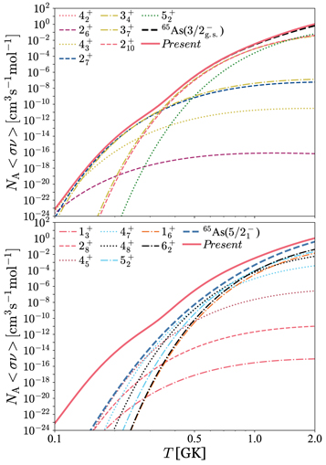
Figure 3. The dominant resonances contributing to the 65As(p,γ)66Se reaction rates. Top panel: the main contributing resonances of proton captures on the  state of 65As. Bottom panel: the main contributing resonances of proton captures on the
  state of 65As. The Present rate (red line) is plotted together with the rates contributed from the proton captures on the
  (black dashed line) and
  (blue dashed line) states of 65As in each panel.
Download figure:
Standard image High-resolution image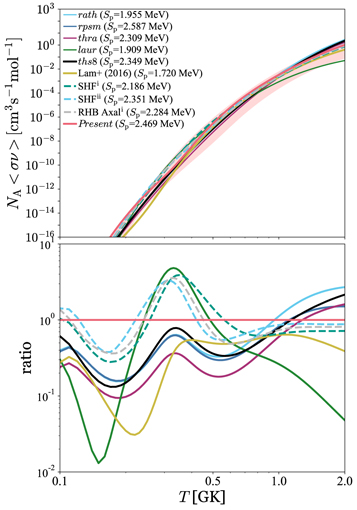
Figure 4. The 65As(p,γ)66Se thermonuclear reaction rates in the temperature region of XRB interest. Top panel: the rath, rpsm, thra, laur, and ths8 are the available rates compiled by Cyburt et al. (2010) and ths8 is the recommended rate published in part of the JINA REACLIB v2.2 release (Cyburt et al. 2010). Lam et al. (2016) rate is based on Sp(66Se) = 1.720 MeV (Audi et al. 2012; AME2012). The uncertainties of the Present rate are indicated as the light red zone. Bottom panel: comparison of the Present rate with all reaction rates presented in the top panel.
Download figure:
Standard image High-resolution imageThe Present reaction rates are presented in Table 2 and the parameters listed in Table 3 can be used to reproduce the Present centroid reaction rate with n = 191, a fitting error of 4.5%, and an accuracy quantity of ζ = 0.003 for the temperature range from 0.1–2 GK according to the format and evaluation procedure proposed by Rauscher & Thielemann (2000). The parameterized rate is obtained using the Computational Infrastructure for Nuclear Astrophysics (CINA; Smith et al. 2004). For the rate above 2 GK, we refer to statistical-model calculations to match with the Present rate, see NACRE (Angulo et al. 1999).
Table 2. Thermonuclear Reaction Rates of 65As(p,γ)66Se
| T9 | Centroid | Lower Limit | Upper Limit |
|---|---|---|---|
| (cm3 s−1 mol−1) | (cm3 s−1 mol−1) | (cm3 s−1 mol−1) | |
| 0.1 | 7.56 × 10⁻²⁴ | 3.53 × 10⁻²⁵ | 2.09 × 10⁻²³ |
| 0.2 | 5.34 × 10⁻¹⁵ | 9.90 × 10⁻¹⁷ | 7.12 × 10⁻¹⁵ |
| 0.3 | 1.13 × 10⁻¹¹ | 1.59 × 10⁻¹² | 6.21 × 10⁻¹¹ |
| 0.4 | 3.61 × 10−09 | 1.96 × 10⁻¹⁰ | 2.04 × 10−08 |
| 0.5 | 3.04 × 10−07 | 7.03 × 10−09 | 8.20 × 10−07 |
| 0.6 | 6.33 × 10−06 | 1.56 × 10−07 | 1.19 × 10−05 |
| 0.7 | 5.63 × 10−05 | 1.94 × 10−06 | 1.01 × 10−04 |
| 0.8 | 2.97 × 10−04 | 1.37 × 10−05 | 5.45 × 10−04 |
| 0.9 | 1.12 × 10−03 | 6.50 × 10−05 | 2.12 × 10−03 |
| 1.0 | 3.38 × 10−03 | 2.32 × 10−04 | 6.46 × 10−03 |
| 1.1 | 8.65 × 10−03 | 6.66 × 10−04 | 1.63 × 10−02 |
| 1.2 | 1.96 × 10−02 | 1.63 × 10−03 | 3.55 × 10−02 |
| 1.3 | 4.01 × 10−02 | 3.50 × 10−03 | 6.90 × 10−02 |
| 1.4 | 7.57 × 10−02 | 6.66 × 10−03 | 1.23 × 10−01 |
| 1.5 | 1.34 × 10−01 | 1.17 × 10−02 | 2.02 × 10−01 |
| 1.6 | 2.22 × 10−01 | 1.90 × 10−02 | 3.13 × 10−01 |
| 1.7 | 3.50 × 10−01 | 2.86 × 10−02 | 4.59 × 10−01 |
| 1.8 | 5.29 × 10−01 | 4.05 × 10−02 | 6.46 × 10−01 |
| 1.9 | 7.68 × 10−01 | 5.53 × 10−02 | 8.75 × 10−01 |
| 2.0 | 1.08 | 7.33 × 10−02 | 1.15 |
Download table as: ASCIITypeset image
Table 3. Parameters a of 65As(p,γ)66Se Centroid Reaction Rate
| i | a0 | a1 | a2 | a3 | a4 | a5 | a6 |
|---|---|---|---|---|---|---|---|
| 1 | −2.98258 × 10+1 | −2.35942 × 10+0 | +3.94649 × 10+0 | −9.86873 × 10+0 | 1.45916 × 10⁻¹ | +1.01711 × 10⁻¹ | 2.46893 × 10+0 |
| 2 | −1.49044 × 10+1 | −3.68082 × 10+0 | +3.93081 × 10+0 | −9.86417 × 10+0 | 1.55748 × 10⁻¹ | +1.02469 × 10⁻¹ | 2.45374 × 10+0 |
| 3 | +1.29861 × 10⁻¹ | −4.94352 × 10+0 | +7.67143 × 10+0 | −2.00710 × 10+1 | 1.29501 × 10+0 | −2.73522 × 10⁻² | 6.16001 × 10+0 |
| 4 | +2.60957 × 10+1 | −1.04676 × 10+1 | +1.64542 × 10+1 | −4.16331 × 10+1 | 3.26017 × 10+0 | −3.38444 × 10⁻¹ | 1.34811 × 10+1 |
| 5 | +3.41675 × 10+1 | −1.41042 × 10+1 | +2.12287 × 10+1 | −5.17133 × 10+1 | 4.54240 × 10+0 | −3.08117 × 10⁻¹ | 1.87553 × 10+1 |
Note.
a The a0,...,a6 parameters are substituted in to reproduce the forward reaction rate with an accuracy quantity,
  , where n is the number of data points, rm
are the original Present rate calculated for each respective temperature, and fm
are the fitted rate at that temperature (Rauscher & Thielemann 2000), see text.
, where n is the number of data points, rm
are the original Present rate calculated for each respective temperature, and fm
are the fitted rate at that temperature (Rauscher & Thielemann 2000), see text.Download table as: ASCIITypeset image
The new reverse 65As(p,γ)66Se reaction rate based on the Sp(66Se) = 2.469 MeV is related to the respective forward reaction rate, Equation (2), via the expression (Rauscher & Thielemann 2000; Schatz & Ong 2017),

where Gi and Gf are the partition functions of initial and final nuclei. The new reverse rates are presented in Figure 5, and compared with the ths8 statistical-model reverse rate. The respective uncertainty (lower and upper limits) of the Present reverse rate corresponds to the uncertainty (lower and upper limits) of the Present forward rate with the consideration of 100 keV uncertainty imposed from the present Sp(66Se). Although this 100 keV uncertainty is rather extreme, its range is capable to cover possible reverse rates due to other estimated Sp(66Se), i.e., Sp(66Se) = 2.433 ± 0.144, 2.443 ± 0.101, and 2.507 ± 0.070 MeV, see Table 1 and Figure 2. The corresponding reverse rates of Sp(66Se) = 2.351 ± 0.144 and 2.284 ±0.092 MeV (cyan and gray dotted lines in Figure 5) are at the upper limit of the Present reverse rate, whereas the reverse rate of Sp(66Se) = 2.186 ± 0.128 MeV (green dotted lines in Figure 5) is about one order of magnitude higher than the Present reverse rate.

Figure 5. The 65As(p,γ)66Se forward and reverse thermonuclear reaction rates in the temperature region of the XRB of interest. Top panel: the ths8 forward and reverse rates are the recommended rates in the JINA REACLIB v2.2 release (Cyburt et al. 2010). The uncertainties of the Present (Sp = 2.469 ± 0.100 MeV) forward and reverse rates are indicated as light red and light pink zones, respectively. Bottom panel: the magnified portion in the top panel for T = 0.8–2 GK.
Download figure:
Standard image High-resolution image3. Implication on One-dimensional Multi-zone GS 1826−24 Clocked Burst Models
We use the Kepler code (Weaver et al. 1978; Woosley et al.2004; Heger et al. 2007) to construct the theoretical XRB models matched with the periodic XRBs, Epoch 1998 June, of the GS 1826−24 X-ray source compiled by Galloway et al. (2017). These XRB models are fully self-consistent. The evolution of chemical inertia and hydrodynamics that power the nucleosynthesis along the rp-process path are correlated with the mutual feedback between the nuclear energy generation in the accreted envelope and the rapidly evolving astrophysical conditions. Meanwhile, the Kepler code uses an adaptive reaction network of which the relevant reactions out of the more than 6000 isotopes from JINA REACLIB v2.2 (Cyburt et al. 2010) are automatically included or discarded throughout the evolution of thermonuclear runaway in the accreted envelope.
The XRB models keep tracking the evolution of a grid of Lagrangian zones, of which each zone has its own isotopic composition and thermal properties. We use the time-dependent mixing length theory (Heger et al. 2000) to describe the convection that transfers synthesized and accreted nuclei and heat between these Lagrangian zones. We remark that this important feature is not considered in zero-dimensional one-zone and post-processing XRB models.
We adopt the astrophysical settings of the GS 1826−24 model from Jacobs et al. (2018) to match with the observed burst light-curve properties of Epoch 1998 June. To obtain the best-matched modeled light-curve profile with the observed profile and averaged recurrence time, Δtrec = 5.14 ± 0.7 h, we assign the accreted 1H, 4He, and CNO metallicity fractions to 0.71, 0.2825, and 0.0075, respectively, whereas the accretion rate is adjusted to a factor of 0.114 of the Eddington-limited accretion rate,  . This refined GS 1826−24 XRB model with JINA REACLIB v2.2 defines the baseline model in this work. Other models that adopt the same astrophysical settings but implement the Present 65As(p,γ)66Se forward and reverse rate (solid and dotted red lines in the top panel of Figure 5), or the lower limit of Present 65As(p,γ)66Se forward and reverse rates (lower borders of red and pink zones in the top panel of Figure 5), or the Present 65As(p,γ)66Se forward and reverse rate (solid and dotted red lines in the top panel of Figure 5) and 22Mg(α,p)25Al (Hu et al. 2021) rates are labeled as the Present†, Present‡, and Present§ models, respectively. These Present†,‡,§ models take into account the recently updated reaction rates around historical 56Ni and 64Ge waiting points, namely, 55Ni(p,γ)56Cu (Valverde et al. 2019), 57Cu(p,γ)58Zn (Lam et al. 2022), 56Ni(p,γ)57Cu (Kahl et al. 2019), and 64Ge(p,γ)65As (Lam et al. 2016) reactions.
We select the latest 22Mg(α,p)25Al reaction rate, which was experimentally deduced by Hu et al. (2021) with the important nuclear structure properties corresponding to the XRB Gamow window instead of the 22Mg(α,p)25Al reaction rate deduced by Randhawa et al. (2020) via direct measurement. This is because the Randhawa et al. (2020) rate was extrapolated from the non-XRB energy region and may have an additional and large uncertainty that was not shown (Hu et al. 2021). The recent direct measurement performed by Jayatissa et al. (2021) could be helpful to further constrain the 22Mg(α,p)25Al reaction rate as long as the measurement directly corresponds to the XRB Gamow window.
We follow the simulation procedure implemented by Lam et al. (2022) and Hu et al. (2021), of which we run a series of 40 consecutive XRBs for the baseline, Present§, Present‡, and Present† models. The first 10 bursts of each model are discarded because these bursts transit from a chemically fresh envelope to an enriched envelope with burned-in burst ashes and stable burning. The burst ashes are recycled in the following burst heatings and stabilize the succeeding bursts. Therefore, we only sum up the last 30 bursts and then average them to produce a modeled burst light-curve profile. This averaging procedure was applied by Galloway et al. (2017) to yield an averaged-observed light-curve profile of Epoch 1998 June, which was recorded by the Rossi X-ray Timing Explorer (RXTE) Proportional Counter Array (Galloway et al. 2004,2008, 2020) and was compiled into the Multi-Instrument Burst Archive 10 by Galloway et al. (2020). Our averaging procedure was also implemented in the works of Lam et al. (2022) and Hu et al. (2021).
3.1. Clocked Bursts of the GS 1826−24 X-Ray Source
The observed flux, Fx, is expressed as (Johnston et al. 2020)  , where Lx is the burst luminosity generated from each model; d is the distance; ξb takes into account the possible deviation of the observed flux from an isotropic burster luminosity (Fujimoto 1988; He & Keek 2016); and the redshift, z, adjusts the light curve when transforming into an observer's frame. Assuming that the anisotropy factors of burst and persistent emissions are degenerate with distance, the d and ξb can be combined to form the modified distance
  . Instead of specifically selecting data close to the burst peak at t = −10 to 40 s as done by Meisel (2018) and Randhawa et al. (2020), we impartially fit the modeled burst light curves generated from each model to the entire burst time span of the averaged-observed light curve to avoid artifactually expanding the modeled burst light curve and shift the modeled burst peak, imposing unknown uncertainty. The best-fit
  and (1 + z) factors of the baseline, Present§, Present‡, and Present† modeled light curves to the averaged-observed light curve and recurrence time of Epoch 1998 June are 7.38 kpc and 1.27, 7.46 kpc and 1.26, 7.34 kpc and 1.28, 7.50 kpc and 1.27, respectively. The averaged-modeled recurrence times of baseline, Present§, Present‡, and Present† are 5.11, 4.97, 5.13, and 5.03 h, respectively. The modeled recurrence times of the baseline and Present‡ scenarios are in good agreement with the observed recurrence time, whereas the modeled recurrence times of the Present§ and Present† scenarios are lower than the observed recurrence time by 0.17 and 0.11 h, respectively, suggesting a 1%–2% decrement can be applied for the accretion rate of the Present§ and Present† models. Such decrement also indicates the new reaction rates used in the Present§ and Present† models shorten up to 3% of the recurrence time.
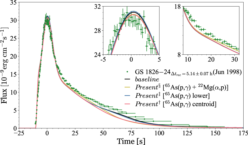
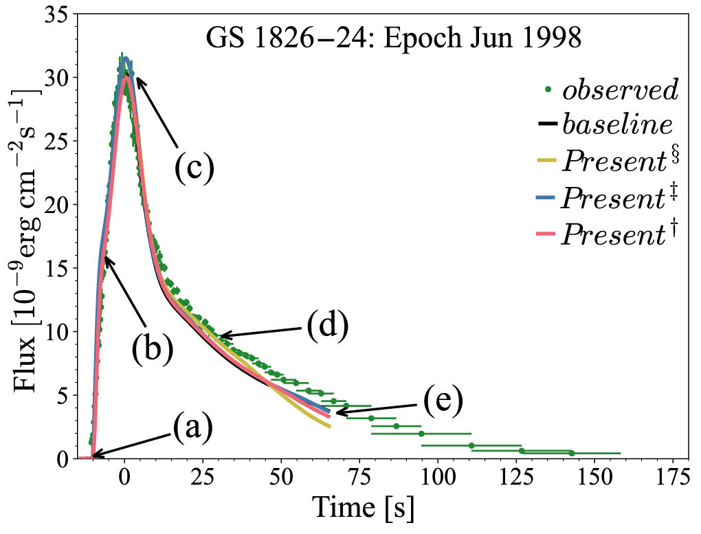
We define the burst-peak time, t = 0 s. The evolution time of the light curve is with respect to the burst-peak time. Figure 6 displays the best-fit modeled and observed XRB light-curve profiles. The observed burst peak is located in the time regime t = −2.5 to 2.5 s (top left inset in Figure 6), and at the vicinity of the modeled light-curve peaks of baseline, Present§, Present‡, and Present†. The overall averaged flux deviations between the observed epoch and each of these theoretical models, baseline, Present§, Present‡, and Present† in units of 10−9 erg cm−2 s−1 are 1.175, 1.159, 1.149, and 1.252, respectively.

Figure 6. The averaged light curves of GS 1826−24 clocked burster as a function of time. Top panel: the best-fit baseline, Present†, Present‡, and Present§ modeled light curves to the observed light curve and recurrence time of Epoch 1998 June. Both insets in the top panel magnify the light-curve portions at t = −5 to 5 s (left inset) and t = 8 to 32 s (right inset).
Download figure:
Standard image High-resolution imageAll modeled light curves are less enhanced than the observed light curve at t = 8–125 s due to the reduction in accretion rate. The updated 59Cu(p,γ)60Zn and 61Ga(p,γ)62Ge reaction rates can induce enhancements at t = 8–30 s and t = 35–125 s, respectively (Y. H. Lam et al. 2022, in preparation), see also the supplemental material in Hu et al. (2021). The Present 65As(p,γ)66Se forward and reverse rates decrease the burst light curve at t = 40–100 s (red line in Figure 6), whereas the lower limit of the Present 65As(p,γ)66Se forward and reverse rates produces a similar burst light-curve profile as baseline (blue and black lines in Figure 6). Note that the lower limit of the Present forward and reverse rates are based on a rather extreme Sp(66Se) uncertainty. The burst tail at t = 50–80 s generated from the 65As(p,γ)66Se forward and reverse rates using Sp(66Se) = 2.433, 2.443, and 2.507 MeV could be just≲10−9 erg cm−2s−1 displaced from the burst tail of the Present† scenario (red line in Figure 6) as long as the newly measured Sp(66Se) is within the range of ∼50 keV close to the present Sp(66Se) = 2.469 MeV. The baseline model that implements the NON-SMOKER 65As(p,γ)66Se forward and reverse rates, can be a reference estimating the influence of the Sp(66Se) = 2.351, 2.381, and 2.284 MeV due to the rather close range of Sp(66Se). Besides, the 65As(p,γ)66Se forward and reverse rates generated from the Sp(66Se) = 2.186 MeV may further enhance the burst tail end to be ∼1 × 10⁻⁹ erg cm−2s−1 higher than the baseline at t =50–80 s. The sensitivity study performed by Cyburt et al. (2016) on the influence of (p,γ) forward reaction rates does not exhibit that the 65As(p,γ)66Se forward rate as being influential, whereas the sensitivity study done by Schatz & Ong (2017) indicates that the 65As(p,γ)66Se reverse rate possibly impacts the burst tail. Our present study with the newly deduced 65As(p,γ)66Se forward and reverse rates shows that the correlated forward and reverse rates characterize the burst tail.
The updated 22Mg(α,p)25Al reaction maintains its role in increasing the burst light curve at t = 16–60 s (yellow line in Figure 6) even correlated influences among dominant reactions are included in the Present§ model. This finding agrees with the preliminary result of Y. H. Lam et al. (2022, in preparation) shown in the supplemental material in Hu et al. (2021).
From t = 130 s onward, the baseline and Present§, ‡,† models successfully reproduce the tail end of the burst light curve of GS 1826−24. The modeled burst tail ends produced by Randhawa et al. (2020) are, however, over expanded, which might be due to a somehow limited observed data that are selected for fitting the modeled burst light curves, see Figure 4 in Randhawa et al. (2020) or in Hu et al. (2021).
3.2. Evolutions of Accreted Envelopes and the Respective Nucleosyntheses
We perform a comprehensive study to understand the microphysics behind the differences among these modeled burst light curves by investigating the evolutions of the accreted envelope regime where nuclei heavier than CNO isotopes are densely synthesized against the evolutions of the respective burst light curves of the 15th, 16th, 16th, and 19th bursts for the baseline, Present§, Present‡, and Present† models, respectively. These selected bursts almost resemble the respective averaged light-curve profile presented in Figure 6. The reference time of the accreted envelope and nucleosynthesis in the following discussion is also relative to the burst peak time, t = 0 s.
The moment before and just before the onset. The preceding burst leaves the accreted envelope with synthesized proton-rich nuclei, which go through β+ decays, and enrich the region around long half-live stable nuclei, e.g., 32S, 36Ar, 40Ca, 60Ni, 64Zn, 68Ge, 72Se, 76Kr, and 80Sr, which are the remnants of waiting points. Meanwhile, the unburned hydrogen nuclei above the base of the accreted envelope keep the stable burning active until the freshly accreted stellar fuel stacks up, increasing the density of the accreted envelope due to the strong gravitational pull from the host neutron star of the GS 1826−24 X-ray source for presetting the thermonuclear runaway conditions of the next XRB.
At time t = −10.2 s, just before the onset of the succeeding XRB, the temperature of the envelope reaches a maximum value of 0.9 GK for the baseline, and Present§,‡,† scenarios, see Figures 7.1–7.4, and 8(a). The 64Ge abundance is around one to five orders of magnitude higher than other surrounding isotopes, whereas the ratio of 68Se to 64Ge abundances is ≈1.7. Meanwhile, the evolution of 64Ge mass fraction in the mass coordinate of the accreted envelope is qualitatively analogous to the 66Se mass fraction. The 64Ge abundance is comparable to the 60Zn and 66Se abundances (solid green, blue, and pink lines in Figure Set 7). These four factors indicate that 64Ge is still a significant waiting point. The reaction flow passes through 68Se and advances to heavier proton-rich nuclei region meanwhile the degenerate envelope is on the brink of the onset of XRB.

Figure 7.
The nucleosynthesis and evolution of the envelope correspond to the 15th burst for the baseline scenario. The cycle is the iteration step of the XRB simulation and the time is relative to the burst peak t = 0 s. The averaged abundances of synthesized nuclei are represented by color tones referring to the right color scale in the nuclear chart of each panel. The black squares are stable nuclei. Bottom right insets of the nuclear chart in each panel: the magnified regions of the NiCu, ZnGa, and GeAs cycles. The arrows are merely used to guide the eyes. Top left insets of the nuclear chart in each panel: the time snapshot of modeled burst light curve. Top right insets in each panel: the corresponding temperature (black dotted line) and density (black dashed line) of each mass zone, referring to the right y-axis, and the abundances of synthesized nuclei, referring to the left y-axis. The abundances of H and He are represented by black and red solid lines, respectively. Bottom right insets in each panel: the averaged mass fractions for each nuclear mass, A. Comparisons of averaged mass fractions between baseline and Present‡,§, † scenarios are presented in Figure 9. (The complete figure set (20 images) is available.)
Download figure:
Standard image High-resolution imageFor the baseline scenario, the 2p-capture on 64Ge waiting point is not yet developed, whereas for the Present‡ scenario, the 2p-capture on 64Ge is weak. The reaction flows of these two scenarios follow the weak GeAs II and sub-GeAs II cycles and mainly break out at 69Se, see Figure 1 for the reaction paths in the GeAs cycles. For the Present§ and Present† scenarios, the 2p-capture on 64Ge has already been established, and the breakout flow at 69Se is rather similar to the baseline and Present‡ scenarios as the 68Se and 69Se abundances for these four scenarios are rather similar. The strong 2p-capture on 64Ge in the Present§ and Present† scenarios causes more than two orders of magnitude of 65As and 66Se cumulated in the GeAs cycles compared to the baseline and Present‡ scenarios (dotted–dashed cyan and dotted dark brown lines in top right insets of each panel in Figures 7.1–7.4). Using either the upper (or lower) limits of the new 64Ge(p,γ)65As reaction rate (Lam et al. 2016) could mildly enhance (or reduce) the strength of 2p-capture on 64Ge of drawing the synthesized materials from 64Ge. Note that the GeAs cycles are still considered weak as compared to the NiCu and ZnGa cycles; nevertheless, the reaction flows in the GeAs cycles of the Present§ and Present† scenarios is stronger than the ones in the baseline and Present‡ scenarios. The high 66Se abundance in the Present§ and Present† scenarios are due to the implementation of the Present 65As(p,γ)66Se forward (and reverse) reaction rate, which is a factor of ∼1.7 higher than (a factor of ∼4.5 lower than) the NON-SMOKER 65As(p,γ)66Se forward (reverse) rate at T = 0.9 GK used in the baseline, and is about two orders (∼1.5 order) of magnitude higher than the lower limit of the Present65As(p,γ)66Se forward (reverse) rate used in the Present‡, see Figure 4.
The moment at t = −7.5 s before the burst peak. Overall the light curves of the baseline, Present‡, Present§, and Present† scenarios rise to 15.4, 16.3, 16.2, and 14.9 in units of 10−9 erg cm−2 s−1, respectively (top left insets of each panel in Figures 7.5–7.8, and Figure 8(b)). The modeled light curve is quantitatively comparable to the observed bolometric flux. As the temperature of the envelope rises to around 1.1 GK, the 2p-capture on 64Ge waiting point and the weak GeAs cycles starts being established in the baseline and Present‡ scenarios, which are about 2.5 s later than the Present§ and Present† scenarios because both 65As(p,γ)66Se rates used in the baseline and Present‡ scenarios are up to (or more than) a factor of 2.5 in T = 0.4–1.1 GK lower than the one used in the Present§ and Present† scenarios (Figure 4). Also, the reverse 65As(p,γ)66Se rate used in the baseline is about a factor of 8.5 higher than the Present reverse rate used in the Present§, ‡,†, causing a rather low cumulation of 66Se in the baseline.

Figure 8. The evolution of a clocked burst for the baseline (15th burst), Present§ (16th burst), Present‡ (16th burst), and Present† (19th burst) with respect to the averaged-observed clocked burst of GS 1826−24 burster, at times (a) t = −10.2 s, (b) t = −7.5 s, (c) t ≈ 0 s, (d) t ≈ 30 s, and (e) t ≈ 65 s. The corresponding comparisons of averaged mass fractions for each mass number at the moments (a), (b), (c), (d), and (e) are presented in Figure 9.
Download figure:
Standard image High-resolution imageThe mass fractions of synthesized nuclei in the GeAs cycles evolve inversely with the rise of the temperature of the envelope along the mass zone, except 66Se (and 65As for the baseline scenario). The evolution of the production of 65As, 66Se, 66As, 67Se, 67As, 68Se, and 68As up to this moment indicates that a strong reaction flow is formed along the 64Ge(p,γ)65As (p,γ)66Se(β+ ν)66As(p,γ)67Se(β+ ν)67As(p,γ)68Se(β+ ν)68As(p,γ)69Se path for these four scenarios. The growth of the 65As mass fraction in the baseline is due to the higher NON-SMOKER 65As(p,γ)66Se reverse rate using Sp(66Se) =2.349 MeV, indicating that some material is temporarily stored as 65As in the baseline scenario. For the Present§, ‡,† scenarios, more material is transmuted from 65As and temporarily stored as 66Se, which then decays via the (β+ ν) channel and quickly transmutes to 69Se and surges through the heavier proton-rich region.
The moment at the vicinity of the burst peak. The accreted envelopes of baseline, Present‡, Present§, and Present† reach the maximum temperature at times −0.9 s (1.33 GK), −1.1 s (1.34 GK), −1.5 s (1.34 GK), and −0.8 s (1.34 GK), respectively. The rise in temperature in the envelope before the burst peak for all scenarios due to the mutual feedback between the nuclear energy generation and hydrodynamics during the onset induces the release of material stored in dominant cycles of nuclei lighter than 64Ge. Due to the lower 65As(p,γ)66Se reaction rates used in the baseline and Present‡, less material is drawn to 68Se causing the production of 64Ge surpasses 68Se in these two scenarios. In fact, both 64Ge and 68Se have already been produced and cumulated when t ≈ −10.6 s or ≈0.5 s before the onset.
The location of the observed burst peak could be ±0.5 s away from the modeled burst peaks of these four scenarios (top left insets of each panel in Figures 7.9–7.12, and Figure 8(c)). Note that the advantage of impartially fitting the whole observed burst light curve helps us to avoid unexpectedly shifting the modeled burst peak further away from the thought location of the observed burst peak. Such misalignment with the observed burst peak occurs in the modeled burst peaks produced by the Randhawa et al. (2020) models, see Figure 4 in Randhawa et al. (2020) or in Hu et al. (2021).
We find that the Present§ model uses the latest 22Mg(α,p)25Al reaction rate (Hu et al. 2021), which extends the dominance of the 22Mg(p,γ)23Al reaction up to 1.67 GK. This causes the reaction flow in the Present§ scenario mainly follows the 22Mg(p,γ)23Al(p,γ)24Si path at the 22Mg branch point that is faster for the reaction flow to synthesize more proton-rich nuclei nearer to the proton dripline than the 22Mg(α,p)25Al(p,γ)26Si path and gives rise to more hydrogen burning at a later time.
The moment at t ≈ 30 s after the burst peak. The consequence of more hydrogen burning caused by the latest 22Mg(α,p)25Al reaction rate, which is almost one order of magnitude lower than the NON-SMOKER 22Mg(α,p)25Al reaction rate, manifests on the enhancement of burst light curve at the time regime t = 16–60 s for the Present§ scenario (top left insets of each panel in Figures 7.13–7.16, and Figure 8(d)). Such enhancement is consistent with that found by Hu et al. (2021), and exhibits the role of important reactions found by Cyburt et al. (2016) improving the modeled burst light curve.
The moment at t ≈ 65 s after the burst peak. The modeled burst light curves diverge at t ≈ 45 s and reach a distinctive difference at t ≈ 65 s (top left insets of each panel in Figures 7.17–7.20 and Figure 8(e)). Materials that have been released since around the burst-peak period from cycles in the sd-shell, e.g., the NeNa, SiP, SCl, and ArK cycles, in the bottom p f-shell, e.g., the CaSc cycle, have passed through the NiCu, ZnGa, and weak GeAs cycles, enrich the region beyond Ge and Se. The 2p-capture on 64Ge for the baseline and Present‡ only lasts until t = 21.4 and 35.8 s, respectively, whereas for Present§ and Present†, this 2p-capture lasts until t = 49.1 s and t = 58.6 s, respectively. The longer time the 2p-capture on 64Ge extends in the XRBs, the more material is transferred via the 64Ge(p,γ)65As(p,γ)66Se(β+ ν)66As(p,γ)67Se(β+ ν)67As(p,α)68Se(β+ ν)68As(p,α)69Se path to surge through the region above Se with intensive (p,γ)-(β+ ν) reaction sequences depleting accreted hydrogen appreciably (solid black lines in the top right inset of each panel in Figures 7.17–7.20). The H exhaustion in the envelope quenches the (p,γ) reactions, reduces the syntheses of proton-rich nuclei, and the produced proton-rich nuclei are left to sequential (β+ ν) decays increasing the production of daughter nuclei, e.g., 62Zn, 66Ge, 60Ni, and 64Zn, which are the daughter nuclei of the ZnGa and GeAs cycles, and 60Zn and 64Ge waiting points.
3.3. Burst Ashes
The baseline and Present§,‡,† models that we construct reproduce the burst tail end of the GS 1826−24 clocked burst from t = 130 s onward with excellent agreement with the averaged-observed Epoch 1998 June. Nevertheless, in the burst tail ends produced by Randhawa et al. (2020) both the baseline and updated model are overexpanded and misaligned with observation (Epoch 2000 September). Such deviation indicates that their modeled burst does not recess in accord with the observation and H-burning may somehow still be active in the envelope. The deviation could also be due to the limited data specifically chosen for fitting the modeled burst light curve or due to the astrophysical settings of both models, see Figure 4 in Randhawa et al. (2020) or in Hu et al. (2021). The one-zone model constructed by Schatz & Ong (2017) successfully estimates a gross feature of the burst light curve influenced by a scaled 65As(p,γ)66Se reaction rate (with Sp(66Se) of 100 keV uncertainty larger than the one used in NON-SMOKER 65As(p,γ)66Se rate); however, the H-burning diminishes earlier than their baseline model due to the extreme parameters implemented (H. Schatz 2021, private communication), causing a more rapid decrease of the burst tail end.
The compositions of burst ashes generated from the baseline and Present§,‡,† models are presented in Figure 9(f). The temperature of the accreted envelope decreases from 0.8–0.64 GK starting from t = 65–150 s. The weak feature of the latest 22Mg(α,p)25Al reaction rate, which is more than two order of magnitudes lower than the 22Mg(p,γ)23Al reaction at T = 0.8–0.64 GK, allows more nuclei to be produced via the 22Mg(p,γ)23Al(p,γ)24Si reaction flow. The material in the reaction flow is then stored in the dominant cycles in sd-shell nuclei, e.g., the SiP, SCl, and ArK cycles. As H is then almost depleted, decreasing nuclear energy generated from (p,γ) reactions and causing the drop in temperature, the reaction flow is less capable to break out from cycles in p f-shell nuclei. The synthesized materials are kept in these cycles until the end of the burst. Therefore, the implementation of the latest 22Mg(α,p)25Al in the Present§ model increases the production of a hot CNO cycle and sd-shell nuclei up to a factor of 4.5 (for 12C which could be the main fuel for the Type I X-ray superburst; Cumming et al. 2006). Meanwhile, compared to the baseline model, the abundance of 12C isotope is increased by about a factor of 4.2 based on the Present‡ model. These nuclei mainly are the remnants (daughter nuclei) left over from the proton-rich nuclei in the dominant cycles of p- and sd-shell nuclei. Such enrichment of sd-shell nuclei enhances the light nuclei abundances that eventually sink to the neutron-star surface.

Figure 9. The averaged mass fractions for each mass number at times (a) t = −10.2 s, (b) t = −7.5 s, (c) t ≈ 0 s, (d) t ≈ 30 s, (e) t ≈ 65 s, and (f) t ≈ 150 s (top panel of each subfigure). The comparison of averaged mass fractions between baseline and Present‡,§, † is presented in the bottom panel of each subfigure.
Download figure:
Standard image High-resolution imageWe notice that a periodic increment exhibits in the remnant of A = 64–88 nuclei up to a factor of 1.4, with a leading increment of waiting points remnants, A = 64, 68, 72, 76, 80, 84, and 88. This indicates that a set of even weaker cycles resembling the weak GeAs II and sub-II cycles exists at waiting points heavier than 68Se. Nonetheless, the 2p-capture on waiting point feature is extremely weak for waiting points heavier than 64Ge, e.g., 68Se, 72Kr, 76Sr, and 80Zr. The periodic increment of Present§ is weaker than Present‡ and Present† because materials are still stored in the dominant cycles of sd-shell nuclei due to the weak 22Mg(α,p)25Al reaction. Moreover, the abundances of nuclei A > 100 decreases for the Present§,‡,† models as more materials are kept in the cycles of sd- and p f-shell nuclei.
3.4. Neutron-star Mass–radius Relation
Using the best-fit modeled burst light curve produced from the baseline and Present§,‡,† models, we estimate  , of which the uncertainty is based on the averaged deviation (2%) of the comparison of the modeled light curves with the averaged-observed light curve of Epoch 1998 June. The range of host neutron-star mass–radius relation, MNS–RNS, of the GS 1826−24 X-ray source is then estimated using our best-fit (1 + z) and Equation (1) of Johnston et al. (2020). The deduced range of MNS–RNS for GS 1826−24 is compared with recently assessed MNS–RNS constraints, i.e., the MNS of PSR J0348+0432 and PSR J1614−2230 deduced by Antoniadis et al. (2013) and Demorest et al. (2010), respectively, based on the Shapiro time delay (overlapping pink strips in Figure 10), the MNS–RNS of PSR J0740+6620 estimated recently by Riley et al. (2021) using Bayesian analysis (green zone in Figure 10), the MNS of PSR J1903+0327 and PSR J1909−3744 compiled by Arzoumanian et al. (2018; distinctive light pink strips in Figure 10), the RNS range of neutron stars with MNS = 1.4, 1.7, and 2M⊙ proposed by Steiner et al. (2018; three yellow lines in Figure 10), the MNS–RNS of GS 1826−24 proposed by Johnston et al. (2020) using the Markov chain Monte-Carlo method to estimate the properties of the three epochs (dark purple line in Figure 10), lower and upper limits of RNS given by Bauswein et al. (2017; black dot in Figure 10), and by Fattoyev et al. (2018; blue dot in Figure 10) based on the study of the GW170817 neutron-star merger.

Figure 10. The MNS–RNS constraints based on observed pulsars with uncertainties δ MNS < 0.05 M⊙: PSR J0348+0432 (Antoniadis et al. 2013), PSR J1614−2230 (Demorest et al. 2010), and PSR J1903+0327 and PSR J1909−3744 (Arzoumanian et al. 2018); Bayesian estimation of MNS–RNS of PSR J0740+6620 (Riley et al. 2021); (1 + z) deduced from the Present§ best-fitted modeled light curve for the GS 1826−24 clocked bursts and from Johnston et al. (2020) based on three epochs; quiescent low-mass X-ray binaries (Guillot et al. 2013), causality Koranda et al. 1997; Lattimer & Prakash 2007, and conditional constraints from the GW170817 neutron-star merger (Bauswein et al. 2017) and realistic models of the equation of state (Fattoyev et al. 2018; Steiner et al. 2018).
Download figure:
Standard image High-resolution image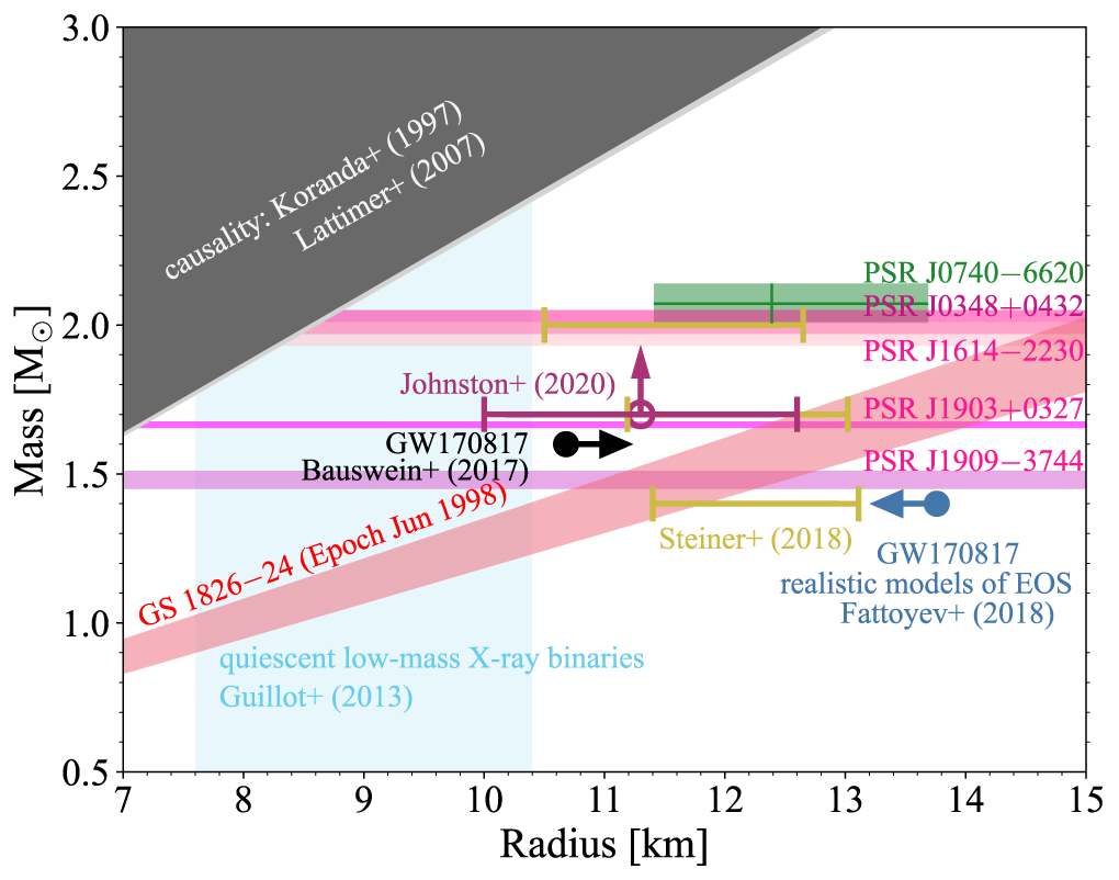
The presently estimated range of MNS–RNS for GS 1826−24 (light red zone in Figure 10) overlaps with the constraints suggested by Johnston et al. (2020) and Steiner et al. (2018) (Figure 10), presuming that its MNS–RNS is likely in the range of MNS ≳ 1.7M⊙ and RNS ∼ 12.4–13.5 km. This suggests that the radius of PSR J1903+0327 could be close to the range of 12.4 ≲ RNS km−1 ≲ 13.5, and neutron stars with MNS ≈ 1.7M⊙ could be less compact than that estimated by Guillot et al.(2013).
We emphasize that as the present neutron-star mass–radius constraint is based on  deduced from XRB models with averaged deviations between modeled and observed burst light curves up to 1.252 × 10⁻⁹ erg cm−2 s−1, a (1 + z) factor deduced from a well-matched modeled and observed burst light curve with much lower deviation is highly desired to provide a more reasonable constraint.
4. Summary and Conclusion
We use the self-consistent RHB theory with DD-ME2 interaction to calculate the MDE for isospin I = 1/2, 1, 3/2, and 2 p f-shell mirror nuclei of A = 41–75. Then, a set of Sp(66Se) values are obtained from folding the experimental 66Geand 65Ge nuclear masses and theoretical MDEs, or the experimental 66Ge and 65As nuclear masses and theoretical MDEs. The Sp(66Se) = 2.469 ± 0.054 MeV is selected to be the reference. The 54 keV uncertainty is deduced from the rms deviation of the comparison of both theoretical and updated experimental MDEs (AME2020). Then, using the full p f-model space shell-model calculations with the GXPF1a Hamiltonian, we choose Sp(66Se) = 2.469 MeV as a reference, and conservatively assume the uncertainty to be 100 keV to estimate the extent of the new 65As(p,γ)66Se forward and reverse reaction rates to cover other estimated Sp(66Se), i.e., Sp(66Se) = 2.433, 2.443, and 2.507 MeV, whereas the forward and reverse reaction rates based on Sp(66Se) = 2.186, 2.351, and 2.284 MeV are calculated as well. We comprehensively study the influence of the new rate on the burst light curve of the GS 1826−24 clocked burster, nucleosynthesis in and evolution of the accreted envelope, and burst-ash abundances at the burst tail end. Future precisely measured Sp(66Se) with uncertainty lower than or ≈50 keV can confirm our present findings and predictions.
We find that the duration of 2p-capture on 64Ge and weak GeAs cycles are affected by the new 65As(p,γ)66Se forward and reverse reaction rates. The longer time the 2p-capture on 64Ge is maintained in a clocked XRB of the GS 1826−24 X-ray source,the more material is transferred via the 64Ge(p,γ)65As(p,γ)66Se(β+ ν)66As(p,γ)67Se(β+ ν)67As(p,α)68Se(β+ ν)68As(p,α)69Se path to reach the region heavier than Se of which intensive (p,γ)–(β+ ν) reaction sequences ascertainably burn accreted hydrogen, release nuclear energy, and thus increase the burst light curve. Meanwhile, the status of 64Ge as an important and historic waiting point is affirmed by analogizing the evolution of 64Ge production with the synthesis of 66Se along the mass coordinate of the accreted envelope, and the comparable abundances of 64Ge, 60Zn, and 66Se in the accreted envelope.
We also include the new 22Mg(α,p)25Al reaction rate in our study, and find that its influence on the clocked XRB at the time regime t = 16–60 s and burst-ash compositions is stronger than other considered reactions, i.e., the new 65As(p,γ)66Se forward and reverse, 56Ni(p,γ)57Cu(p,γ)58Zn, 55Ni(p,γ)56Cu, and 64Ge(p,γ)65As reactions. The affected burst-ash compositions consist of nuclei in hot CNO cycle, sd and p f shells, up to A = 140, except A = 87,...,96. Both the Present§ and Present† models show that the abundances of nuclei A = 64, 68, 72, 76, and 80 are affected up to a factor of 1.4. The inclusion of the updated 22Mg(α,p)25Al reaction rate in Present§ influences the production of 12C up to a factor of 4.5 that could be the main fuel for the superburst. A set of noticeably periodic increments of burst-ash abundances exists in the region heavier than 64Ge with waiting points leading the increment, indicating that the resemblance of 2p-capture and weak GeAs cycles also coexists in the region during the thermonuclear runaway.
We remark that the impartial fit on the whole time span of the burst light curve permits us to produce a set of modeled burst light curves with excellent agreement with the observed Epoch 1998 June at the burst peak and tail end, and the distinguishing feature of the light curve is reproduced. The averaged deviation between modeled and observed burst light is only up to 1.252 × 10⁻⁹ erg cm−2 s−1. The best-fit modeled bursts, which diminish accordingly with observation and with considerably low discrepancy, presumably provide a set of more convincing burst-ash abundances that are not observed. This permits us to understand the nucleosyntheses that happen during the thermonuclear runaway in the accreted envelope. The modeled burst light curve produced by Randhawa et al. (2020) is, however, rather extensive and the H-burning does not recede accordingly with observation, and also the modeled burst peak is misaligned with observation. The one-zone model constructed by Schatz & Ong (2017) successfully obtains the influence of the 65As(p,γ)66Se reaction rate (with larger Sp(66Se) compared to the NON-SMOKER 65As(p,γ)66Se rate) on a gross feature of a burst light curve; however, the H-burning recedes earlier than their baseline model, accelerating the recession of the burst tail end.
In this work, we presume the radius of the host neutron star of GS 1826−24 to be in the range of ∼12.4–13.5 km as long as its mass ≳1.7M⊙. Besides, the radius of PSR J1903+0327 could likely be close to the range of 12.4 ≲ RNS km−1 ≲ 13.5, and future observations could shed light on the estimation of neutron-star radii coupled with MNS ≈ 1.7M⊙. This presumption indicates that the neutron-star compactness estimated by Guillot et al. (2013) is somehow more compact.
We are deeply grateful to H. Schatz for reading our manuscript and for providing thoughtful and constructive suggestions to improve the manuscript, and to B. A. Brown for providing the previous and updated Sp(66Se) and for reading and suggesting constructive thoughts to the part related to the Sp(66Se). We thank W. J. Huang for providing the information of AME. We also thank the anonymous referee for the helpful comments and remarks on this manuscript. We are very thankful to N. Shimizu for suggestions in tuning the KShell code at the PHYS_T3 (Institute of Physics) and QDR4 clusters (Academia Sinica Grid-computing Centre) of Academia Sinica, Taiwan, to D. Kahl for checking and implementing the newly updated 56Ni(p,γ)57Cu reaction rate, to M. Smith for using the Computational Infrastructure for Nuclear Astrophysics, and to J. J. He for fruitful discussion. This work was financially supported by the Strategic Priority Research Program of the Chinese Academy of Sciences (CAS, Grant Nos. XDB34000000 and XDB34020204) and the National Natural Science Foundation of China (No. 11775277). We are appreciative of the computing resource provided by the Institute of Physics (PHYS_T3 cluster) and the Academia Sinica Grid-computing Center (ASGC) Distributed Cloud resources (QDR4 cluster) of Academia Sinica, Taiwan. Part of the numerical calculations was performed at the Gansu Advanced Computing Center. Y.H.L. gratefully acknowledges the financial support from the Chinese Academy of Sciences President's International Fellowship Initiative (No. 2019FYM0002) and appreciates the laptop (Dell M4800) partially sponsored by Pin-Kok Lam and Fong-Har Tang during the COVID-19 pandemic. A.H. is supported by the Australian Research Council Centre of Excellence for Gravitational Wave Discovery (OzGrav, No. CE170100004) and for All Sky Astrophysics in 3 Dimensions (ASTRO 3D, No. CE170100013). A.H., A.M.J., and Z.J. were supported, in part, by the US National Science Foundation under Grant No. PHY-1430152 (JINA Center for the Evolution of the Elements, JINA-CEE).