


Abstract
The nearby (3.8 Mpc) galaxy NGC 4945 hosts a nuclear starburst and Seyfert type 2 active galactic nucleus (AGN). We use the Atacama Large Millimeter/submillimeter Array (ALMA) to image the 93 GHz (3.2 mm) free–free continuum and hydrogen recombination line emission (H40α and H42α) at 2.2 pc (0 12) resolution. Our observations reveal 27 bright, compact sources with FWHM sizes of 1.4–4.0 pc, which we identify as candidate super star clusters. Recombination line emission, tracing the ionizing photon rate of the candidate clusters, is detected in 15 sources, six of which have a significant synchrotron component to the 93 GHz continuum. Adopting an age of ∼5 Myr, the stellar masses implied by the ionizing photon luminosities are
  (M⋆/M⊙) ≈ 4.7–6.1. We fit a slope to the cluster mass distribution and find β = −1.8 ± 0.4. The gas masses associated with these clusters, derived from the dust continuum at 350 GHz, are typically an order of magnitude lower than the stellar mass. These candidate clusters appear to have already converted a large fraction of their dense natal material into stars and, given their small freefall times of ∼0.05 Myr, are surviving an early volatile phase. We identify a pointlike source in 93 GHz continuum emission that is presumed to be the AGN. We do not detect recombination line emission from the AGN and place an upper limit on the ionizing photons that leak into the starburst region of Q0 < 1052 s−1.
Export citation and abstract BibTeX RIS

Original content from this work may be used under the terms of the Creative Commons Attribution 4.0 licence. Any further distribution of this work must maintain attribution to the author(s) and the title of the work, journal citation and DOI.
1. Introduction
Many stars form in clustered environments (Lada & Lada 2003; Kruijssen 2012). Bursts of star formation with high gas surface density produce massive (>105 M⊙), compact (FWHM size of 2–3 pc; Ryon et al. 2017) clusters, referred to as super star clusters. Super star clusters likely have high star formation efficiencies (Goddard et al. 2010; Adamo et al. 2011; Ryon et al. 2014; Adamo et al. 2015; Johnson et al. 2016; Chandar et al. 2017; Ginsburg & Kruijssen 2018). They may represent a dominant output of star formation during the peak epoch of star formation (z ∼ 1–3; Madau & Dickinson 2014). The process by which these massive clusters form may now also relate to the origin of globular clusters.
The earliest stages of cluster formation are the most volatile and currently unconstrained (Dale et al. 2015; Ginsburg et al. 2016; Krause et al. 2016; Li et al. 2019; Krause et al. 2020). Characterizing properties of young (<10 Myr) clusters is a key step toward understanding their formation, identifying the dominant feedback processes at each stage of cluster evolution, determining which clusters survive as gravitationally bound objects, and linking all of these processes to the galactic environment.
While young clusters of mass ∼104 M⊙ are found within our Galaxy (Bressert et al. 2012; Longmore et al. 2014; Ginsburg et al. 2018), the most massive young clusters in the local universe are often found in starbursting regions and merging galaxies (e.g., Zhang & Fall 1999; Whitmore et al. 2010; Linden et al. 2017). Direct optical and even near-infrared observations of forming clusters are complicated by large amounts of extinction. Analyses of optically thin free–free emission and long-wavelength hydrogen recombination lines of star clusters offer an alternative, extinction-free probe of the ionizing gas surrounding young star clusters (Condon 1992; Roelfsema & Goss 1992; Murphy et al. 2018). However, achieving a spatial resolution matched to the size of young clusters  (1 pc) (Ryon et al. 2017) in galaxies at the necessary frequencies and sensitivities has only recently become possible thanks to the Atacama Large Millimeter/submillimeter Array (ALMA).
We have recently analyzed forming super star clusters in the central starburst of the nearby (3.5 Mpc) galaxy NGC 253 at ∼2 pc resolution (Leroy et al. 2018; E.A.C. Mills et al. 2020, in preparation). The galaxy NGC 4945 is the second object we target in a campaign to characterize massive star clusters in local starbursts with ALMA.
The galaxy NGC 4945 is unique in that it is one of the closest galaxies (3.8 ± 0.3 Mpc; Karachentsev et al. 2007) where a detected active galactic nucleus (AGN) and central starburst coexist. In the central ∼200 pc, the starburst dominates the infrared luminosity and ionizing radiation (Marconi et al. 2000; Spoon et al. 2000 ), and an outflow of warm ionized gas has been observed (Heckman et al. 1990; Moorwood et al. 1996; Mingozzi et al. 2019). Individual star clusters have not previously been observed in NGC 4945 due to the high extinction at visible and short IR wavelengths (e.g., AV ≳ 36 mag; Spoon et al. 2000). Evidence for a Seyfert AGN comes from strong, variable X-ray emission, as NGC 4945 is one of the brightest sources in the X-ray sky and has a Compton thick column density of 3.8 × 1024 cm−2 (Marchesi et al. 2018). A kinematic analysis of H2O maser emission yields a black hole mass of 1.4 × 10⁶ M⊙ (Greenhill et al. 1997).
In this paper, we use ALMA to image the 93 GHz free–free continuum and hydrogen recombination line emission (H40α and H42α) at 2.2 pc (012) resolution. This emission allows us to probe photoionized gas on star cluster scales and thereby trace ionizing photon luminosities. We identify candidate star clusters and estimate properties relating to their size, ionizing photon luminosity, stellar mass, and gas mass.
Throughout this paper, we plot spectra in velocity units with respect to a systemic velocity of Vsystematic = 580 km s−1 in the local standard of rest frame; estimates of the systemic velocity vary by ±25 km s−1 (e.g., Chou et al. 2007; Roy et al. 2010; Henkel et al. 2018). At a distance of 3.8 Mpc, 01 corresponds to 1.84 pc.
2. Observations
We used the ALMA Band 3 receivers to observe NGC 4945 as part of the project 2018.1.01236.S (PI: A. Leroy). We observed NGC 4945 with the main 12 m array telescopes in intermediate and extended configurations. Four spectral windows in Band 3—centered at 86.2, 88.4, 98.4, and 100.1 GHz—capture the millimeter continuum primarily from free–free emission and cover the hydrogen recombination lines of principal quantum number (to the lower state)  and 42 from the α (
 ) transitions. The rest frequency of H40α is 99.0230 GHz, and that of H42α is 85.6884 GHz.
In this paper, we focus on the 93 GHz (λ ∼ 3.2 mm) continuum emission and the recombination line emission arising from compact sources in the starbursting region. We image the data from an 8 km extended configuration, which are sensitive to spatial scales of 007–6'' (2–100 pc), in order to focus on the compact structures associated with candidate clusters. We analyze the observatory-provided calibrated visibilities using version 5.4.0 of the Common Astronomy Software Application (CASA; McMullin et al. 2007).
When imaging the continuum, we flag channels with strong spectral lines. Then we create a continuum image using the full bandwidth of the line-free channels. We also make continuum images for each spectral window. For all images, we use Briggs weighting with a robust parameter of r = 0.5.
When imaging the two spectral lines of interest, we first subtract the continuum in uv space through a first-order polynomial fit. Then, we image by applying a CLEAN mask (to all channels) derived from the full-bandwidth continuum image. Again, we use Briggs weighting with a robust parameter of r = 0.5, which represents a good compromise between resolution and surface brightness sensitivity.
After imaging, we convolved the continuum and line images to convert from an elliptical to a round beam shape. For the full-bandwidth continuum image presented in this paper, the fiducial frequency is ν = 93.2 GHz, and the final FWHM beam size is θ = 012. The rms noise away from the source is ≈0.017 mJy beam−1, equivalent to 0.2 K in Rayleigh–Jeans brightness temperature units. Before convolution to a round beam, the beam had a major and minor FWHM of 0097 × 0071.
For the H40α and H42α spectral cubes, the final FWHM beam size is 020, convolved from 0097 × 0072 and 011 × 0083, respectively. The slightly lower resolution resulted in more sources with significantly detected line emission. We boxcar-smoothed the spectral cubes from the native 0.488 MHz channel width to 2.93 MHz. The typical rms in the H40α cube is 0.50 mJy beam−1 per 8.9 km s−1 channel. The typical rms in the H42α cube is 0.48 mJy beam−1 per 10.3 km s−1 channel.
As part of the analysis, we compare the high-resolution data with observations taken in a 1 km intermediate configuration as part of the same observing project. We use the intermediate-configuration data to trace the total recombination line emission of the starburst. We use the continuum image provided by the observatory pipeline, which we convolve to have a circular beam FWHM of 07; the rms noise in the full-bandwidth image is 0.15 mJy beam−1. The spectral cubes have a typical rms per channel of 0.24 mJy beam−1 with the same channel widths as the extended-configuration cubes. We do not jointly image the configurations because our main science goals are focused on compact, pointlike objects. The extended-configuration data on their own are well suited to study these objects, and any spatial filtering of extended emission will not affect the analysis.
We compare the continuum emission at 3 mm with archival ALMA imaging of the ν = 350 GHz (λ ∼ 850 μm) continuum (project 2016.1.01135.S; PI: N. Nagar). At this frequency, dust emission dominates the continuum. We imaged the calibrated visibilities with a Briggs robust parameter of r = −2 (toward uniform weighting), upweighting the extended baselines to produce a higher-resolution image suitable for comparison to our new Band 3 data. We then convolve the images to produce a circularized beam, resulting in an FWHM resolution of 012 (from an initial beam size of 010 × 0064), exactly matched to our 93 GHz continuum image. These data have an rms noise of 0.7 mJy beam−1 (0.2 K).
We compare the ALMA data with Australian Long Baseline Array (LBA) imaging of ν = 2.3 GHz continuum emission (Lenc & Tingay 2009). At this frequency and resolution, the radio continuum is predominantly synchrotron emission. We use the Epoch 2 images (courtesy of E. Lenc) that have a native angular resolution slightly higher than the 3 mm ALMA data, with a beam FWHM of 0080 × 0032 and an rms noise of 0.082 mJy beam−1.
3. Continuum Emission
The whole disk of NGC 4945, as traced by Spitzer IRAC 8 μm emission (program 40410; PI: G. Rieke), is shown in Figure 1. The 8 μm emission predominantly arises from UV-heated polycyclic aromatic hydrocarbons (PAHs), thus tracing the interstellar medium and areas of active star formation. The black square indicates the 8'' × 8'' (150 pc × 150 pc) starburst region that is of interest in this paper.

Figure 1. Spitzer IRAC 8 μm emission from UV-heated PAHs over the full galactic disk of NGC 4945. The black square indicates the 8'' × 8'' (150 pc × 150 pc) central starburst region of interest in this paper; the inset shows the ALMA 93 GHz continuum emission.
Download figure:
Standard image High-resolution imageFigure 2 shows the 93 GHz (λ ∼ 3 mm) continuum emission in the central starburst of NGC 4945. Our image reveals ∼30 peaks of compact, localized emission with peak flux densities of 0.6–8 mJy (see Section 3.1). On average, the continuum emission from NGC 4945 at this frequency is dominated by thermal, free–free (bremsstrahlung) radiation (Bendo et al. 2016). Free–free emission from bright, compact regions may trace photoionized gas in the immediate surroundings of massive stars. We take into consideration the pointlike sources detected at 93 GHz as candidate massive star clusters, though some contamination by synchrotron-dominated supernova remnants or dusty protoclusters may still be possible. The morphology of the 93 GHz emission and clustering of the peaks indicate possible ridges of star formation and shells. The extended, faint negative bowls flanking the main disk likely reflect the short spacing data missing from this image. We do not expect that they affect our analysis of the point source–like cluster candidates.

Figure 2. ALMA 93 GHz (λ ∼ 3.2 mm) continuum emission in the central starburst of NGC 4945. The continuum at this frequency is dominated by ionized, free–free emitting plasma. In this paper, we show that the pointlike sources are primarily candidate massive star clusters. The brightest point source of emission at the center is presumably the Seyfert AGN. The rms noise away from the source is σ ≈ 0.017 mJy beam−1, and the circularized beam FWHM is 012 (or 2.2 pc at the distance of NGC 4945). The contours of the continuum image show 3σ emission (gray) and [4σ, 8σ, 16σ, ... 256σ] emission (black).
Download figure:
Standard image High-resolution imageThe large amount of extinction present in this high-inclination central region (i ∼ 72°; Henkel et al. 2018) has previously impeded the direct observation of its star clusters. The Paschen-α (Paα) emission (Marconi et al. 2000) of the  hydrogen recombination line at 1.87 μm, shown in Figure 3, reveals faint emission above and below the star-forming plane. Corrected for extinction, the clumps of ionized emission traced by Paα would give rise to free–free emission below our ALMA detection limit. The Paα and mid-infrared (MIR) spectral lines give support for dust extinction of AV > 160 mag surrounding the AGN core and more generally AV ≳ 36 mag in the star-forming region (Spoon et al. 2000).

Figure 3. Top left: 93 GHz continuum emission with sources identified; also see Table 1. Circles show apertures (diameter of 024) used for continuum extraction. Their colors indicate the measured in-band spectral index, as in Figure 4, where dark purple indicates synchrotron-dominated emission and yellow indicates dust-dominated emission. Top right: HST Paα emission–hydrogen recombination line,  , at 1.87 μm (courtesy of P. van der Werf) tracing ionized gas at ≈02 resolution (Marconi et al. 2000). Dust extinction of AV > 36 mag obscures the Paα recombination emission at shorter wavelengths from the starburst region. Contours trace 93 GHz continuum, as described in Figure 2. Bottom left: ALMA 350 GHz continuum emission tracing dust. Bottom right: Australian LBA 2.3 GHz continuum imaging of synchrotron emission primarily from supernova remnants (Lenc & Tingay 2009).
Download figure:
Standard image High-resolution imageA large fraction (18/29) of the 93 GHz sources coincide with peaks in dust emission at 350 GHz, as shown in Figure 3. Overall, there is a good correspondence between the two tracers. This indicates that candidate clusters are relatively young and may still harbor reservoirs of gas, though in Section 5.7, we find that the fraction of the mass still in gas tends to be relatively small.
In Figure 3, the 93 GHz peaks without dust counterparts tend to be strong sources of emission at 2.3 GHz (Lenc & Tingay 2009), a frequency where synchrotron emission typically dominates. As discussed in Lenc & Tingay (2009), the sources at this frequency are predominantly supernova remnants. The presence of 13 possible supernova remnants—four of which are resolved into shell-like structures 1.1–2.1 pc in diameter—indicates that a burst of star formation activity started at least a few Myr ago. Lenc & Tingay (2009) modeled the spectral energy distributions (SEDs) of the sources spanning 2.3–23 GHz and found significant opacity at 2.3 GHz (τ = 5–22), implying the presence of dense, free–free plasma in the vicinity of the supernova remnants.
At 93 GHz, the very center of the starburst shows an elongated region of enhanced emission (about 20 pc in projected length, or ∼1'') that is also bright in 350 GHz emission. This region is connected to the areas of highest extinction. Higher column densities of ionized plasma are also present in the region; Lenc & Tingay's (2009) observations reveal large free–free opacities, at least up to 23 GHz. The brightest peak at 93 GHz, centered at (α, δ)93 = (13 h 05 m 27.4798 s ± 0.004 s, −49° 28' 05.404'' ± 0.06''), is colocated with the kinematic center as determined from H2O maser observations  = (13 h 05 m 27.279 s ± 0.02s, −49° 28' 04.44'' ± 0.1'') (Greenhill et al. 1997) and presumably harbors the AGN core. We refer to the elongated region of enhanced emission surrounding the AGN core as the circumnuclear disk. The morphological similarities between 93 and 350 GHz, together with the detection of a synchrotron point source (likely a supernova remnant; see Section 3.2 and source 17) in the circumnuclear disk, indicate that star formation is likely present there.
3.1. Point-source Identification
We identify candidate star clusters via pointlike sources of emission in the 93 GHz continuum image. Sources are found using PyBDSF (Mohan & Rafferty 2015) in the following way. Islands are defined as contiguous pixels (of nine pixels or more) above a threshold of seven times the global rms value of σ ≈ 0.017 mJy beam−1. Within each island, multiple Gaussians may be fit, each with a peak amplitude greater than the peak threshold of 10 times the global rms. We chose this peak threshold to ensure that significant emission can also be identified in the continuum images made from individual spectral windows. The number of Gaussians is determined from the number of distinct peaks of emission higher than the peak threshold that have a negative gradient in all eight evaluated directions. Starting with the brightest peak, Gaussians are fit and cleaned (i.e., subtracted). A source is identified with a Gaussian as long as subtracting its fit does not increase the island rms.
Applying this algorithm to our 93 GHz image yielded 50 Gaussian sources. We remove five sources that fall outside of the star-forming region. We also remove three sources that appeared blended, with an offset <012 from another source. Finally, we remove 13 sources that do not have a flux density above 10 times the global rms after extracting the 93 GHz continuum flux density through aperture photometry (see Section 3.2). As a result, we analyze 29 sources as candidate star clusters. In Figure 3, we show the location of each source with the apertures used for flux extraction. The sources match well with what we would identify by eye.
3.2. Point-source Flux Extraction
For each source, we extract the continuum flux density at 2.3, 93, and 350 GHz through aperture photometry. Before extracting the continuum flux at 2.3 GHz, we convolve the image to the common resolution of 012. We extract the flux density at the location of the peak source within an aperture diameter of 024. Then we subtract the extended background continuum that is local to the source by taking the median flux density within an annulus of inner diameter 024 and outer diameter 030; using the median suppresses the influence of nearby peaks and the bright surrounding filamentary features. The flux density of each source at each frequency is listed in Table 1. When the extracted flux density within an aperture is less than three times the global rms noise (in the 2.3 and 350 GHz images), we assign a 3σ upper limit to that flux measurement.
Table 1. Properties of the Continuum Emission from Candidate Star Clusters
| Source | R.A. | Decl. | S93 | α93 | S2.3a | S350b | fff | fsync | fdc |
|---|---|---|---|---|---|---|---|---|---|
| (mJy) | (mJy) | (mJy) | |||||||
| 1 | 13:05:27.761 | −49:28:02.83 | 1.28 ± 0.13 | −0.80 ± 0.11 | 2.3 ± 0.4 | ⋯ | 0.51 ± 0.08 | 0.49 | ⋯ |
| 2 | 13:05:27.755 | −49:28:01.97 | 1.01 ± 0.10 | 0.80 ± 0.22 | ⋯ | 26.6 | 0.78 ± 0.05 | ⋯ | 0.22 |
| 3 | 13:05:27.724 | −49:28:02.64 | 0.82 ± 0.08 | −0.27 ± 0.23 | ⋯ | 14.8 | 0.89 ± 0.16 | 0.11 | ⋯ |
| 4 | 13:05:27.662 | −49:28:03.85 | 0.95 ± 0.09 | −1.12 ± 0.42 | ⋯ | 16.0 | 0.27 ± 0.31 | 0.73 | ⋯ |
| 5 | 13:05:27.630 | −49:28:03.76 | 0.77 ± 0.08 | −1.57 ± 0.63 | ⋯ | ⋯ | 0.00 ± 0.40 | 1.00 | ⋯ |
| 6 | 13:05:27.612 | −49:28:03.35 | 1.73 ± 0.17 | −1.11 ± 0.22 | 7.1 ± 0.7 | ⋯ | 0.28 ± 0.16 | 0.72 | ⋯ |
| 7 | 13:05:27.602 | −49:28:03.15 | 0.98 ± 0.10 | −0.61 ± 0.19 | ⋯ | 15.5 | 0.65 ± 0.14 | 0.35 | ⋯ |
| 8 | 13:05:27.590 | −49:28:03.44 | 1.89 ± 0.19 | −0.40 ± 0.20 | ⋯ | 14.9 | 0.80 ± 0.15 | 0.20 | ⋯ |
| 9 | 13:05:27.571 | −49:28:03.78 | 1.76 ± 0.18 | −1.01 ± 0.22 | 12.2 ± 1.2 | ⋯ | 0.36 ± 0.16 | 0.64 | ⋯ |
| 10 | 13:05:27.558 | −49:28:04.77 | 2.41 ± 0.24 | −1.10 ± 0.20 | 9.5 ± 0.9 | ⋯ | 0.29 ± 0.14 | 0.71 | ⋯ |
| 11 | 13:05:27.557 | −49:28:03.60 | 0.76 ± 0.08 | −0.59 ± 0.38 | ⋯ | 13.9 | 0.66 ± 0.28 | 0.34 | ⋯ |
| 12 | 13:05:27.540 | −49:28:03.99 | 1.28 ± 0.13 | 1.47 ± 0.37 | ⋯ | 37.4 | 0.62 ± 0.09 | ⋯ | 0.38 |
| 13 | 13:05:27.530 | −49:28:04.27 | 1.78 ± 0.18 | −0.22 ± 0.15 | ⋯ | 20.8 | 0.93 ± 0.11 | 0.07 | ⋯ |
| 14 | 13:05:27.528 | −49:28:04.63 | 3.06 ± 0.31 | −1.22 ± 0.19 | 14.3 ± 1.4 | 11.2 | 0.20 ± 0.14 | 0.80 | ⋯ |
| 15 | 13:05:27.522 | −49:28:05.80 | 0.83 ± 0.08 | −0.71 ± 0.28 | ⋯ | ⋯ | 0.57 ± 0.21 | 0.42 | ⋯ |
| 16 | 13:05:27.503 | −49:28:04.08 | 0.98 ± 0.10 | 1.34 ± 0.37 | ⋯ | 23.9 | 0.65 ± 0.09 | ⋯ | 0.35 |
| 17 | 13:05:27.493 | −49:28:05.10 | 3.69 ± 0.37 | −0.61 ± 0.13 | 5.3 ± 0.5 | 47.1 | 0.65 ± 0.10 | 0.35 | ⋯ |
| 18 | 13:05:27.480 | −49:28:05.40 | 9.74 ± 0.97 | −0.85 ± 0.05 | ⋯ | 39.0 | 0.47 ± 0.03 | 0.53 | ⋯ |
| 19 | 13:05:27.464 | −49:28:06.55 | 1.30 ± 0.13 | −1.36 ± 0.38 | 7.8 ± 0.8 | ⋯ | 0.10 ± 0.28 | 0.90 | ⋯ |
| 20 | 13:05:27.457 | −49:28:05.76 | 2.51 ± 0.25 | −0.88 ± 0.13 | ⋯ | 22.4 | 0.45 ± 0.09 | 0.55 | ⋯ |
| 21 | 13:05:27.366 | −49:28:06.92 | 1.19 ± 0.12 | −1.38 ± 0.41 | 4.7 ± 0.5 | ⋯ | 0.09 ± 0.30 | 0.91 | ⋯ |
| 22 | 13:05:27.358 | −49:28:06.07 | 2.57 ± 0.26 | −0.19 ± 0.18 | ⋯ | 34.8 | 0.95 ± 0.13 | 0.05 | ⋯ |
| 23 | 13:05:27.345 | −49:28:07.44 | 0.95 ± 0.09 | −0.28 ± 0.25 | ⋯ | 9.7 | 0.88 ± 0.18 | 0.12 | ⋯ |
| 24 | 13:05:27.291 | −49:28:07.10 | 0.90 ± 0.09 | −1.22 ± 0.36 | 3.2 ± 0.4 | ⋯ | 0.20 ± 0.26 | 0.80 | ⋯ |
| 25 | 13:05:27.288 | −49:28:06.56 | 0.91 ± 0.09 | −0.27 ± 0.35 | 2.1 ± 0.4 | 15.2 | 0.89 ± 0.26 | 0.11 | ⋯ |
| 26 | 13:05:27.285 | −49:28:06.72 | 1.13 ± 0.11 | −0.33 ± 0.38 | 1.4 ± 0.4 | 18.5 | 0.85 ± 0.28 | 0.15 | ⋯ |
| 27 | 13:05:27.269 | −49:28:06.60 | 2.75 ± 0.28 | −1.08 ± 0.14 | 31.2 ± 3.1 | ⋯ | 0.30 ± 0.10 | 0.70 | ⋯ |
| 28 | 13:05:27.242 | −49:28:08.43 | 0.80 ± 0.08 | −0.54 ± 0.12 | ⋯ | ⋯ | 0.70 ± 0.09 | 0.30 | ⋯ |
| 29 | 13:05:27.198 | −49:28:08.22 | 1.43 ± 0.14 | −0.29 ± 0.20 | ⋯ | 12.6 | 0.88 ± 0.14 | 0.12 | ⋯ |
Notes. Here R.A. and decl. refer to the center location of a Gaussian source identified in the 93 GHz continuum image in units of hour angle and degrees, respectively; S93 is the flux density in the 93 GHz full-bandwidth continuum image; α93 is the spectral index at 93 GHz (S ∝ να), as determined from the best-fit slope to the 85–101 GHz continuum emission; S2.3 is the flux density extracted in the 2.3 GHz continuum image; S350 is the flux density extracted in the 350 GHz continuum image; and fff, fsyn, and fd are the free–free, synchrotron, and dust fractional contribution to the 93 GHz continuum emission, respectively, as determined from the spectral index. See Section 3.3 for a description of how the errors on these fractional estimates are determined.
aA 3σ upper limit to the sources undetected in 2.3 GHz continuum emission is 1.2 mJy. bThe error on the 350 GHz flux density measurement is 3.2 mJy. A 3σ upper limit to the undetected sources is 9.6 mJy. cThe error on the fractional contributions is the same as for fff unless otherwise noted.Download table as: ASCIITypeset image
In Figure 4, we plot the ratio of the flux densities extracted at 350 and 93 GHz (S350/S93) against the ratio of the flux densities extracted at 2.3 and 93 GHz (S2.3/S93). Synchrotron-dominated sources, which fall to the bottom right of the plot, separate from the free–free- (and dust-) dominated sources, which lie in the middle of the plot. One exception is the AGN (source 18), which, due to self-absorption at frequencies greater than 23 GHz, is bright at 93 GHz but not at 2.3 GHz and therefore has the lowest S2.3/S93 ratio.

Figure 4. Top: ratio of the flux densities extracted at 350 and 93 GHz (S350/S93) plotted against the ratio of the flux densities extracted at 2.3 and 93 GHz (S2.3/S93). Bottom: the relation we use to determine the free–free fraction from the in-band index, α93, at 93 GHz. Data points in both plots are colored by the in-band index derived only from our ALMA data. Yellow indicates dust-dominated sources, whereas purple indicates synchrotron-dominated sources. Candidate star clusters in which free–free emission dominates at 93 GHz appear ∼pink. The diameter of each data point is proportional to the flux density at 93 GHz and correspondingly inversely proportional to the error of the in-band spectral index.
Download figure:
Standard image High-resolution imageFrom the continuum measurements, we construct simple SEDs for each source. These SEDs are used for illustrative purposes and do not affect the analysis in this paper. Examples of the SEDs of three sources are included in Figure 5. We show an example of a free–free-dominated source (source 22), which represents the majority of sources, as well as a dust- (source 12) and a synchrotron- (source 14) dominated source. Of the sources with extracted emission of >3σ at 2.3 GHz, nine also have the free–free absorption of their synchrotron spectrum modeled. We plot this information whenever possible. When a source identified by Lenc & Tingay (2009) lies within 006 (half the beam FWHM) of the 93 GHz source, we associate the low-frequency modeling with the 93 GHz source. We take the model fit by Lenc & Tingay (2009) and normalize it to the 2.3 GHz flux that we extract; as an example, see the solid purple curve in the middle panel of Figure 5. The SEDs of all sources are shown in Figure 13 in Appendix C.

Figure 5. Example SEDs constructed for each source. Top: dust-dominated, source 12. Middle: synchrotron-dominated, source 14. Bottom: free–free-dominated, source 22. The dashed orange line represents a dust spectral index of α = 4.0, normalized to the flux density we extract at 350 GHz (orange data point). The dashed black line represents a free–free spectral index of α = −0.12, normalized to the flux density we extract at 93 GHz (black data point). The pink data points show the flux densities extracted from the Band 3 spectral windows. The gray shaded region is the 1σ error range of the Band 3 spectral index fit, except we have extended the fit in frequency for displaying purposes. The purple line represents a synchrotron spectral index of α = −1.5, normalized to the flux density we extract at 2.3 GHz (purple data point), except for source 14, where the solid purple line represents the normalized 2.3–23 GHz fit from Lenc & Tingay (2009). Error bars on the flux density data points are 3σ.
Download figure:
Standard image High-resolution image3.3. Free–Free Fraction at 93 GHz
The flux density of optically thin, free–free emission at millimeter wavelengths (see Appendix A.2; Draine 2011) arises as

where EMC = nen+V is the volumetric emission measure of the ionized gas, D is the distance to the source, and Te is the electron temperature of the medium. Properties of massive star clusters (i.e., ionizing photon rate) can thus be derived through an accurate measurement of the free–free flux density and an inference of the volumetric emission measure. We will determine a free–free fraction, fff, and let Sff = fffS93.
In this section, we focus on determining the portion of free–free emission that is present in the candidate star clusters at 93 GHz. To do this, we need to estimate and remove contributions from synchrotron emission and dust continuum. We determine an in-band spectral index across the 15 GHz bandwidth of the ALMA Band 3 observations. Using the spectral index,12 we constrain the free–free fraction, as well as the fractional contributions of synchrotron and dust (see Figure 4 and Table 1). We found the in-band index to give stronger constraints and, for 2.3 GHz, be more reliable than extrapolating (assuming indices of −0.8, −1.5) because of the two decades' difference in frequency coupled with the large optical depths already present at 2.3 GHz.
3.3.1. Band 3 Spectral Index
We estimate an in-band spectral index at 93 GHz, α93, from a fit to the flux densities in the spectral window continuum images of the ALMA Band 3 data. The spectral windows span 15 GHz, which we set up to have a large fractional bandwidth. We extract the continuum flux density of each source in each spectral window using aperture photometry with the same aperture sizes as described in Section 3.2. We fit a first-order polynomial to the five continuum measurements—four from each spectral window and one from the full-bandwidth image. The fit to the in-band spectral index is listed in Table 1 with the 1σ uncertainty to the fit. The median uncertainty of the spectral indices is 0.13. The spectral indices measured in this way were consistent for the brightest sources with the index determined by CASA tclean; however, we found our method to be more reliable for the fainter sources. Nonetheless, the errors are large for faint sources.
3.3.2. Decomposing the Fractional Contributions of Emission Type
From the in-band spectral index fit, we estimate the fractional contribution of each emission mechanism—free–free, synchrotron, and (thermal) dust—to the 93 GHz continuum. To do this, we simulate how mixtures of synchrotron, free–free, and dust emission could combine to create the observed in-band index. We assume fixed spectral indices for each component and adjust their fractions to reproduce the observations (see below).
We consider that a source is dominated by two types of emission (a caveat we discuss in detail in Section 6): free–free and dust or free–free and synchrotron. With synthetic data points, we first set the flux density at 93 GHz, S93, to a fixed value and vary the contributions of dust and free–free continua, such that S93 = Sd + Sff. For each model, we determine the continuum flux at each frequency across the Band 3 frequency coverage as the sum of the two components. We assume that the frequency dependence of the free–free component is αff = −0.12 and the frequency dependence of the dust component is αd = 4.0. We fit the (noiseless) continuum of the synthetic data across the Band 3 frequency coverage with a power law, determining the slope as α93, the in-band index. We express the results in terms of free–free and dust fractions, rather than absolute flux. In this respect, we explore free–free fractions to the 93 GHz continuum ranging from fff = (0.001, 0.999) in steps of 0.001. We let the results of this process constrain our free–free fraction when the in-band index measured in the actual (observed) data is α93 ≥ −0.12.
Next, we repeat the exercise, but we let synchrotron and free–free dominate the contribution to the continuum at 93 GHz. We take the frequency dependence of the free–free component as αff = −0.12 across the Band 3 frequency coverage, and we set the synchrotron component to αsyn = −1.5. We let the results of this process constrain the free–free fraction of the candidate star clusters when the fit to their in-band index is α93 ≤ −0.12.
Our choices for the spectral indices of the three emission types are motivated as follows. In letting αff = −0.12, we assume that the free–free emission is optically thin (e.g., see Appendix A.2). We do not expect significant free–free opacity at 93 GHz given the somewhat-evolved age of the candidate clusters in the starburst (see Section 5.2). In letting αd = 4.0, we assume the dust emission is optically thin with a wavelength-dependent emissivity so that τ ∝ λ−2 (e.g., see Draine 2011). The low dust optical depths estimated in Section 5.6 imply a dust spectral index steeper than 2, though the exact value might not be 4, e.g., if our assumed emissivity power-law index is not applicable. The generally faint dust emission indicates that our assumptions about dust do not have a large effect on our results. For the synchrotron frequency dependence, we assume αsyn = −1.5. This value is consistent with the best-fit slope of αsyn = −1.4 found by Bendo et al. (2016) averaged over the central 30'' of NGC 4945. Furthermore, the median slope of synchrotron-dominated sources modeled at 2.3–23 GHz is −1.11 (Lenc & Tingay 2009), indicating that even at 23 GHz, the synchrotron spectra already show losses due to aging, i.e., are steeper than a canonical initial injection of αsyn ≈ −0.8. While our assumed value of αsyn = −1.5 is well motivated, on average, variations from source to source are likely present.
Through this method of decomposition, the approximate relation between the in-band index and the free–free fraction is

for which α93 ≤ −0.12, the synchrotron fraction is found to be fsyn = 1 − fff and we set fd = 0, and for which α93 ≥ −0.12 the dust fraction is found to be fd = 1 − fff and fsyn = 0. This relation is depicted in the bottom panel of Figure 4 using the values that have been determined for each source.
3.3.3. Estimated Free–Free, Synchrotron, and Dust Fractions to the 93 GHz Continuum
Table 1 and Figure 4 summarize our estimated fractional contribution of each emission mechanism to the 93 GHz continuum of each source. We use the same relation above to translate the range of uncertainty on the spectral index to an uncertainty in the emission fraction estimates. We find that, at this 012 resolution, the median free–free fraction of sources is fff = 0.62, with a median absolute deviation of 0.29. Most of the spectral indices are negative, and as a result, we find that synchrotron emission can have a nontrivial contribution with a median fraction of fsyn = 0.36 and median absolute deviation of 0.32. On the other hand, three of the measured spectral indices are positive. The median dust fraction of sources is fd = 0 with a median absolute deviation of 0.10. A 1σ limit on the fractional contribution of dust does not exceed fd = 0.47 for any single source.
Additional continuum observations of comparable resolution at frequencies between 2 and 350 GHz would improve the estimates of the fractional contribution of free–free, dust, and synchrotron to the 93 GHz emission.
4. Recombination Line Emission
Hydrogen recombination lines at these frequencies trace ionizing radiation (E > 13.6 eV); this recombination line emission is unaffected by dust extinction. The integrated emission from a radio recombination line transition to quantum number  , which we derive for millimeter-wavelength transitions in Appendix A.1, is described by

where  is the local thermodynamic equilibrium (LTE) departure coefficient, EML = nenpV is the volumetric emission measure of ionized hydrogen, D is the distance to the source, Te is the electron temperature of the ionized gas, and ν is the rest frequency of the spectral line.
Figure 6 shows the spectra of the 15 sources with detected radio recombination line emission. We extract H40α and H42α spectra at the location of each source with an aperture diameter of 04, or twice the beam FWHM. We average the spectra of the two transitions together to enhance the signal-to-noise ratio of the recombination line emission. To synthesize an effective H41α profile, we interpolate the two spectra of each source to a fixed velocity grid with a channel width of 10.3 km s−1; weight each spectrum by  , where σrms is the spectrum standard deviation; and average the spectra together, lowering the final noise. The averaged spectrum has an effective transition of H41α at νeff = 92.034 GHz.

Figure 6. Radio recombination line spectra for sources with significantly detected emission. The thin blue line is the H40α spectrum. The thin green line is the H42α spectrum. These spectra have been regridded from their native velocity resolution to the common resolution of 10.3 km s−1. The thick black line is the weighted average spectrum of H40α and H42α, effectively H41α. In red is the best fit to the effective H41α radio recombination line feature.
Download figure:
Standard image High-resolution imageWe fit spectral features with a Gaussian profile. We calculate an integrated signal-to-noise ratio for each line by integrating the spectrum across the Gaussian width of the fit (i.e., ±σGaus) and then dividing by the noise over the same region,  , where N is the number of channels covered by the region. We report on detections with an integrated signal of >5σrms. Table 2 summarizes the properties of the line profiles derived from the best-fit Gaussian. The median rms of the spectra is σrms = 0.34 mJy.
Table 2. Average Line Profiles Nominally Located Near H41α
| Source | Vcen | Peak | FWHM | σrms |
|---|---|---|---|---|
| (km s−1) | (mJy) | (km s−1) | (mJy) | |
| 1 | 131.6 ± 12 | 0.69 ± 0.16 | 105.2 ± 28 | 0.35 |
| 3 | 117.4 ± 4.0 | 1.26 ± 0.28 | 37.2 ± 9.4 | 0.36 |
| 4 | 107.5 ± 4.3 | 1.28 ± 0.26 | 42.9 ± 10 | 0.36 |
| 6 | 79.4 ± 3.1 | 1.33 ± 0.27 | 31.1 ± 7.3 | 0.33 |
| 7 | 77.2 ± 3.0 | 1.46 ± 0.32 | 28.1 ± 7.0 | 0.36 |
| 8 | 87.5 ± 2.1 | 2.24 ± 0.24 | 38.7 ± 4.9 | 0.33 |
| 12 | 53.6 ± 3.9 | 1.72 ± 0.24 | 55.9 ± 9.1 | 0.39 |
| 13 | 45.7 ± 1.7 | 2.68 ± 0.26 | 34.8 ± 3.9 | 0.31 |
| 14 | 111.8 ± 12 | 0.82 ± 0.12 | 163.1 ± 28 | 0.33 |
| 15 | 5.6 ± 2.8 | 1.62 ± 0.33 | 28.2 ± 6.6 | 0.37 |
| 21 | −140.7 ± 8.3 | 0.99 ± 0.15 | 113.3 ± 20 | 0.34 |
| 22 | −80.6 ± 4.0 | 1.61 ± 0.22 | 58.4 ± 9.4 | 0.34 |
| 25 | −102.3 ± 3.3 | 1.42 ± 0.24 | 39.0 ± 7.7 | 0.32 |
| 26 | −107.6 ± 2.2 | 1.86 ± 0.27 | 30.9 ± 5.3 | 0.33 |
| 27 | −102.3 ± 1.6 | 2.02 ± 0.27 | 23.6 ± 3.6 | 0.28 |
Note. Here Vcen is the central velocity of the best-fit Gaussian, peak is the peak amplitude of the Gaussian fit, FWHM is the FWHM of the Gaussian fit, and σrms is the standard deviation of the fit-subtracted spectrum.
Download table as: ASCIITypeset image
In Figure 12 of Appendix B, we show that the central velocities of our detected recombination lines are in good agreement with the kinematic velocity expected of the disk rotation. To do this, we overlay our spectra on H40α spectra extracted from the intermediate-configuration observations (07 resolution).
In 12 of the 15 sources, we detect relatively narrow features of FWHM ∼ (24–58) km s−1. Larger line widths of FWHM ∼ (105–163) km s−1 are observed from bright sources that also have high synchrotron fractions, indicating that multiple components, unresolved motions (e.g., from expanding shells or galactic rotation), or additional turbulence may be present. Six sources with detected recombination line emission have considerable (fsyn ≳ 0.50) synchrotron emission (i.e., sources 1, 4, 6, 14, 21, and 27) at 93 GHz.
In the top panel of Figure 7, we show the total recombination line emission extracted from the starburst region in the 02 resolution "extended" configuration observations. The aperture we use, designated as region T1, is shown in Figure 8. Details of the aperture selection are described in Section 4.1.1. The spectrum consists of two peaks reminiscent of a double horn profile representing a rotating ring. We fit the spectrum using the sum of two Gaussian components. In Table 3, we include the properties of the best-fit line profiles. The sum total area of the fits is (2.1 ± 0.6) Jy km s−1.

Figure 7. The H40α line spectra extracted from the aperture regions T1 (top) and T2 (bottom; see Figure 8). In blue is the extended-configuration ("extended") spectrum extracted from the high-resolution 02 data; this spectrum shows the maximum total integrated line flux extracted. In purple is the intermediate-configuration ("intermed") spectra extracted from low-resolution, native 07 data; the spectrum from the T2 region is the total maximum integrated line flux from these data. The solid black line represents the sum total of two Gaussian fits. The dotted black line represents the single Gaussian fits.
Download figure:
Standard image High-resolution image
Figure 8. Integrated intensity (moment 0) map of H40α emission integrated at Vsystemic ± 170 km s−1 and observed with the intermediate telescope configuration at native 07 resolution. Overlaid are contours of the 93 GHz continuum from extended-configuration, high-resolution (012) data as described in Figure 1. Red ellipses mark the apertures used to extract the total line emission from regions T1 and T2.
Download figure:
Standard image High-resolution imageTable 3. H40α Line Profiles from the Regions of Total Flux
| Region | Config. | Vcen,1 | Peak1 | FWHM1 | Vcen,2 | Peak2 | FWHM2 | H40α Flux |
|---|---|---|---|---|---|---|---|---|
| (km s−1) | (mJy) | (km s−1) | (km s−1) | (mJy) | (km s−1) | (mJy km s−1) | ||
| T1 | Extended | −139 ± 9 | 9.7 ± 2 | 78 ± 22 | 91 ± 13 | 8.9 ± 1.8 | 138 ± 14 | 2100 ± 600 |
| T1 | Intermed | −117 ± 9 | 16 ± 3 | 99 ± 21 | 66 ± 2 | 16 ± 2 | 186 ± 15 | 4800 ± 900 |
| T2 | Intermed | −114 ± 13 | 19 ± 4 | 113 ± 31 | 86 ± 13 | 23 ± 3 | 167 ± 14 | 6400 ± 1000 |
Download table as: ASCIITypeset image
4.1. Line Emission from 07 Resolution, Intermediate-configuration Observations
Figure 7 also shows integrated spectra derived from intermediate-resolution (07) data. We use these data as a tracer of the total ionizing photons of the starburst region. We expect that the intermediate-resolution data include emission from both discrete, pointlike sources and diffuse emission from any smooth component.
The total integrated emission in the intermediate-configuration data is about three times larger than the integrated emission in the extended-configuration data. Spectra representing the total integrated line flux are shown in Figure 7. In Figure 8, we show the integrated intensity map of H40α emission from the intermediate-configuration (07) data. In Table 3, we include the best-fit line profiles.
We also compare the line profiles of H40α and H42α in the intermediate-configuration (07) data; see Table 4 and Figures 9 and 10. We find that the integrated line emission of H42α is enhanced compared with H40α, reaching a factor of 2 greater when integrated over the entire starburst region. Yet we see good agreement between the two lines at the scale of individual cluster candidates. Spectral lines (possibly arising from c-C3H2) likely contaminate the H42α line flux in broad, typically spatially unresolved line profiles.

Figure 9. Continuum emission at 93 GHz observed with an intermediate configuration with native resolution FWHM = 07 (or 12.9 pc at the distance of NGC 4945). The rms noise away from the source is σ ≈ 0.15 mJy beam−1. The contours of the continuum image show 3σ emission (gray) and [4σ, 8σ, 16σ, ...] emission (black). Apertures (red) with a diameter of 4'' mark the regions N, C, and S.
Download figure:
Standard image High-resolution image
Figure 10. Comparison of our H40α (purple) and H42α (green) from intermediate-configuration, low-resolution data from the regions defined in Figure 9 as N (top), C (middle), and S (bottom). We find H42α to be contaminated by spectral lines that may include c-C3H2 432 − 423, shown as a dashed line in the panels at expected velocities with respect to H42α. When contaminant lines are included, the integrated line flux of H42α is overestimated by a factor of 1.5 in these apertures; this grows to a factor of 2 when integrating over the total starburst emission.
Download figure:
Standard image High-resolution imageTable 4. Comparison of Integrated Recombination Line Flux
| Region | H42α Flux | H40α Flux | Ratio H42α/H40α |
|---|---|---|---|
| (Jy km s−1) | (Jy km s−1) | ||
| N | 2.1 ± 0.2 | 1.5 ± 0.2 | 1.4 ± 0.2 |
| C | 5.9 ± 0.3 | 3.7 ± 0.3 | 1.6 ± 0.2 |
| S | 1.9 ± 0.2 | 0.96 ± 0.1 | 2.0 ± 0.3 |
Download table as: ASCIITypeset image
4.1.1. Total Emission from the Starburst Region
In Figure 8, we show the integrated intensity map of H40α emission integrated in vsystemic ± 170 km s−1 as calculated from the 07 intermediate-configuration data. Diffuse emission is detected throughout the starburst region and up to 30 pc in apparent size beyond the region where we detect the bright point sources at high resolution.
Also shown in Figure 8 are the apertures used to extract spectra in Figure 7. We fit a two-dimensional Gaussian to the continuum emission in the 07 resolution observations (see Figure 9). This results in a best fit centered at (α, δ) = (13hr 05m 27 4896, −49° 28' 05159), with major and minor Gaussian widths of σmaj = 24 and σmin = 058 and an angle of θ = 49
 5; we use this fit as a template for the aperture location, position angle, width, and height. We independently vary the major and minor axes (in multiples of 0.5σmaj and 0.5σmin, respectively) in order to determine the aperture that maximizes the total integrated signal in channels within ±170 km s−1. With the extended-configuration cube, we find the largest integrated line emission with an aperture of 84 × 15, which we refer to as T1. With the intermediate-configuration cube, the largest integrated line emission arises with an aperture of 120 × 29, which we refer to as T2.
We extract the total H40α line flux from the intermediate-configuration (07 resolution) cube using the T2 aperture (see bottom panel of Figure 7). The spectrum shows a double horn profile, indicating ordered disklike rotation. We fit the features with two Gaussians. The sum total of their integrated line flux is (6.4 ± 1.0) Jy km s−1.
We also extract H40α line flux from the intermediate-configuration (07 resolution) cube within the T1 aperture in order to directly compare the integrated line flux in the two different data sets using the same aperture regions. We find more emission in the intermediate-configuration data, a factor of ∼2.3 greater than the extended-configuration data. This indicates that some recombination line emission originates on large scales (>100 pc) to which the high-resolution long baselines are not sensitive.
4.1.2. H42α Contamination
In this section, we compare the line profiles from H40α and H42α extracted from the 07 intermediate-configuration data. In principle, we expect the spectra to be virtually identical, which is why we average them to improve the signal-to-noise ratio at high resolution. Here we test that assumption at low resolution. To summarize, we find evidence that a spectral line may contaminate the H42α measured line flux in broad (typically spatially unresolved) line profiles. Yet we see good agreement between the two lines at the scale of individual cluster candidates.
We extracted spectra in three apertures to demonstrate the constant velocity offset of the contaminants. We approximately matched the locations of these apertures to those defined in Bendo et al. (2016), in which H42α was analyzed at 23 resolution; in this way, we are able to confirm the flux and line profiles we extract at 07 resolution with those at 23. The nonoverlapping circular apertures with diameters of 4'' designated as north (N), center (C), and south (S) are shown in Figure 9.
We used our intermediate-configuration data to extract an H40α and H42α spectrum in each of the regions. We overplot the spectra of each region in Figure 10. We fit a single Gaussian profile to the line emission, except for the H42α emission in region N, where two Gaussian components better minimized the fit. The total area of the fits is presented in Table 4 as the integrated line flux.
Our line profiles of H42α are similar in shape and velocity structure to those analyzed in Bendo et al. (2016), and the integrated line emission is also consistent (within 2σ). This indicates that we are recovering the H42α total line flux and properties with our data.
On the other hand, the H40α flux we extract is about a factor of ∼1.6 lower than the H42α fluxes in these apertures (see Figure 10 and Table 4). The discrepancy grows to a factor of 2 in the profile extracted from the total region.
The additional emission seen in the H42α spectrum at velocities of +100 to +250 km s−1 with respect to the bright, presumably hydrogen recombination line peak is absent in the H40α profile. It is not likely to be a maser-like component of hydrogen recombination emission, since the relative flux does not greatly vary in different extraction regions, and densities outside of the circumnuclear disk would not approach the emission measures necessary (e.g., EMv ≳ 1010 cm−6 pc3) for stimulated line emission.
We searched for spectral lines in the frequency range νrest ∼ 85.617–85.660 GHz corresponding to these velocities and find several plausible candidates, though we were not able to confirm any species with additional transitions in the frequency coverage of these observations. A likely candidate may be the 432 − 423 transition of c-C3H2. This molecule has a widespread presence in the diffuse interstellar medium (ISM) of the Galaxy (e.g., Lucas & Liszt 2000), and the 220 − 211 transition has been detected in NGC 4945 (Eisner et al. 2019). As an example, we plot the velocity of c-C3H2 432 − 423 relative to H42α in Figure 10.
5. Physical Properties of the Candidate Star Clusters
In this section, we estimate the properties of the candidate star clusters, summarized in Table 6. We discuss their size and approximate age. Properties of the ionized gas content, such as temperature (see Table 5), metallicity, density, and mass, are derived from the continuum and recombination line emission. We estimate the ionizing photon rate of the candidate star clusters and use it to infer the stellar mass (see Figure 11). From the dust emission at 350 GHz, we estimate the gas masses of the candidate star clusters. With a combined total mass from gas and stars, we estimate current mass surface densities and freefall times.

Figure 11. Top: complementary cumulative distribution of the ionizing photon rate, Q0, of candidate star clusters in NGC 4945 (see Table 6) and NGC 253 (E.A.C. Mills et al. 2020, in preparation). The turnoff at lower values likely reflects completeness limits. Bottom: stellar mass, M⋆, of our candidate star clusters inferred from the ionizing photon rates of a cluster with an age of 5 Myr, plotted as a complementary cumulative distribution. We also include the stellar masses of clusters in the starburst of NGC 253 (E.A.C. Mills et al. 2020, in preparation) and the galaxies LMC, M51, and the Antennae (Mok et al. 2020). Since the clusters in NGC 253 are likely close to a zero-age main sequence, they would produce more ionizing photons per unit mass as compared with the slightly older stellar population in the clusters of NGC 4945.
Download figure:
Standard image High-resolution imageTable 5. Temperature Analysis
| Source |

|
S93 | fff | Te |
|---|---|---|---|---|
| (mJy km s−1) | (mJy) | (K) | ||
| 8 | 92 ± 15 | 3.5 ± 0.4 | 0.74 ± 0.20 | 6000 ± 1700 |
| 13 | 99 ± 14 | 2.9 ± 0.3 | 0.91 ± 0.22 | 5600 ± 1400 |
| 22 | 100 ± 21 | 3.4 ± 0.3 | 0.78 ± 0.20 | 5600 ± 1700 |
| 26 | 61 ± 13 | 2.6 ± 0.3 | 0.72 ± 0.29 | 6400 ± 2600 |
| 27 | 50 ± 10 | 3.6 ± 0.4 | 0.45 ± 0.16 | 6500 ± 2300 |
Note. Here  refers to the integrated line emission, S93 is the continuum flux density extracted at 93 GHz in the 02 resolution image, fff is the estimated free–free fraction at 02 resolution, and Te is the electron temperature derived using Equation (4).
Download table as: ASCIITypeset image
We exclude source 5 from the analysis, since the free–free fraction is fff < 0.01. We also remove the presumed AGN core (source 18) from the analysis.
5.1. Size
The sources identified through PyBDSF in the 93 GHz continuum image are fit with two-dimensional Gaussians. The average of the major and minor (convolved) FWHM is listed in Table 6 as the FWHM size of the source in units of parsecs. The Gaussian fits are all consistent with circular profiles within the errors. We find FWHM sizes of (1.4–4.0) pc, consistent with the typical sizes of young massive star clusters (Ryon et al. 2017; Leroy et al. 2018). However, the lower end may reflect the resolution limit of our beam, with an FWHM size of 2.2 pc. The uncertainties we report reflect the errors of the Gaussian fit.
Table 6. Physical Properties of Candidate Star Clusters
| Source | FWHM |
 a
a
|
 a
a
|
 a
a
|
 a
a
|
 a
a
|
 a
a
|
 a
a
|
|---|---|---|---|---|---|---|---|---|
| (pc) | (cm−6 pc3) | (cm−6 pc3) | (s−1) | (M⊙) | (M⊙) | (M⊙ pc−2) | (yr) | |
| 1 | 3.0 ± 0.1 | 8.1 | 8.6 | 51.2 | 5.1 | <4.5 | 4.0 | 4.9 |
| 2 | 2.6 ± 0.1 | 8.2 | ⋯ | 51.3 | 5.2 | 4.8 | 4.3 | 4.7 |
| 3 | 3.1 ± 0.1 | 8.2 | 8.4 | 51.2 | 5.2 | 4.8 | 4.1 | 4.9 |
| 4 | 2.5 ± 0.1 | 7.7 | 8.5 | 50.8 | 4.7 | 4.6 | 4.0 | 4.9 |
| 6 | 2.9 ± 0.1 | 8.0 | 8.4 | 51.1 | 5.0 | <4.5 | 3.8 | 5.0 |
| 7 | 2.7 ± 0.1 | 8.1 | 8.4 | 51.2 | 5.1 | 4.6 | 4.2 | 4.8 |
| 8 | 2.4 ± 0.1 | 8.5 | 8.7 | 51.5 | 5.5 | 4.5 | 4.5 | 4.6 |
| 9 | 2.4 ± 0.1 | 8.1 | ⋯ | 51.2 | 5.1 | <4.3 | 4.1 | 4.8 |
| 10 | 2.9 ± 0.1 | 8.2 | ⋯ | 51.2 | 5.1 | <4.5 | 4.0 | 4.9 |
| 11 | 1.4 ± 0.1 | 8.0 | ⋯ | 51.1 | 5.0 | 4.0 | 4.6 | 4.5 |
| 12 | 2.7 ± 0.1 | 8.2 | 8.7 | 51.3 | 5.2 | 5.0 | 4.4 | 4.7 |
| 13 | 2.5 ± 0.1 | 8.5 | 8.7 | 51.6 | 5.5 | 4.7 | 4.6 | 4.6 |
| 14 | 2.2 ± 0.1 | 8.1 | 8.9 | 51.2 | 5.1 | 4.4 | 4.3 | 4.7 |
| 15 | 2.5 ± 0.1 | 8.0 | 8.4 | 51.0 | 5.0 | <4.4 | 4.0 | 4.9 |
| 16 | 2.3 ± 0.1 | 8.1 | ⋯ | 51.2 | 5.1 | 4.7 | 4.3 | 4.7 |
| 17 | 3.1 ± 0.1 | 8.7 | ⋯ | 51.7 | 5.7 | 5.2 | 4.6 | 4.6 |
| 19 | 2.4 ± 0.1 | 7.4 | ⋯ | 50.5 | 4.4 | <4.3 | 3.5 | 5.1 |
| 20 | 3.7 ± 0.1 | 8.4 | ⋯ | 51.4 | 5.3 | 5.1 | 4.2 | 4.9 |
| 21 | 3.1 ± 0.1 | 7.3 | 8.8 | 50.4 | 4.3 | <4.6 | 3.1 | 5.4 |
| 22 | 2.4 ± 0.1 | 8.7 | 8.7 | 51.8 | 5.7 | 4.9 | 4.8 | 4.5 |
| 23 | 2.6 ± 0.1 | 8.2 | ⋯ | 51.3 | 5.2 | 4.4 | 4.3 | 4.7 |
| 24 | 3.1 ± 0.1 | 7.6 | ⋯ | 50.6 | 4.6 | <4.6 | 3.4 | 5.2 |
| 25 | 3.9 ± 0.2 | 8.2 | 8.5 | 51.3 | 5.2 | 5.0 | 4.0 | 5.0 |
| 26 | 3.4 ± 0.1 | 8.3 | 8.5 | 51.3 | 5.3 | 4.9 | 4.2 | 4.9 |
| 27 | 2.2 ± 0.1 | 8.2 | 8.4 | 51.3 | 5.2 | <4.3 | 4.3 | 4.7 |
| 28 | 4.0 ± 0.1 | 8.0 | ⋯ | 51.1 | 5.0 | <4.8 | 3.6 | 5.1 |
| 29 | 2.9 ± 0.1 | 8.4 | ⋯ | 51.5 | 5.4 | 4.6 | 4.3 | 4.7 |
Note. Source 5 is not included because its free–free fraction is fff < 0.01; source 18 is not included because it is the AGN core. The FWHM is the source size as best fit from a Gaussian (to flux that has not been deconvolved); the errors reflect the fit of the Gaussian. Here EMC is the free–free emission measure derived from the continuum as in Equation (1), and EML is the hydrogen free–free emission measure derived from effective H41α as in Equation (3); we note EMC = (1 + y)EML. Here Q0 is the ionizing photon rate derived from EMC as in Equation (7), and M⋆ is the stellar mass derived from Q0 as in Equation (8).
aThe error on these quantities is ∼0.4 dex.Download table as: ASCIITypeset image
Based on high-resolution imaging of embedded clusters in the nucleus of the Milky Way and NGC 253, some of these clusters might break apart at higher resolution (Ginsburg et al. 2018, Levy et al., in preparation). If they follow the same pattern seen in these other galaxies, each source would have one or two main components with potentially several associated fainter components.
5.2. Age
Throughout our analysis, we assume that the candidate star clusters formed in an instantaneous burst of star formation roughly 5 Myr ago (with a likely uncertainty of ∼1 Myr). This (approximately uniform) age is supported through the coincident detection of radio recombination lines (RRLs) and supernova remnants, previous analyses of the global population of the burst (e.g., Marconi et al. 2000; Spoon et al. 2000), and an orbital timescale of ≈3 Myr for the starburst region. We elaborate on this supporting evidence below.
As we discuss in Section 3.3, dust does not significantly contribute to 93 GHz emission (with a median fraction of fd = 0), but synchrotron emission does through supernova remnants. Supernova explosions begin from ∼3 Myr in the lifetime of a cluster and cease at about ∼40 Myr, when the most massive stars have died out; this puts the loosest bounds on the age of the candidate clusters we observe. The coincident detection of supernova remnants in one-third (6/15) of our recombination line–detected sources implies that the burst is likely not at the earliest stage of the supernova phase. However, the ionizing photon rate changes dramatically over 3–10 Myr, dropping by about two orders of magnitude (Leitherer et al. 1999). As a result, clusters are significantly harder to detect in radio recombination lines or free–free continuum emission after ∼5 Myr.
Properties of star-forming activity in the central starburst have been estimated by combining far-infrared (FIR) and optical/IR tracers. Marconi et al. (2000) discerned an age of 6 Myr and mass of 4 × 10⁷ M⊙ by using Paα and Brγ to trace the energy distribution of the photon output of the population. However, the dust extinction was underestimated, complicated by the uncertainty in the AGN contribution. The MIR observations of line ratios with the Infrared Space Observatory (ISO; Kessler et al. 1996) further constrained this scenario. Spoon et al. (2000) estimated an extinction of AV = 36 + 18−11, determined that the AGN is not dominating the ionizing radiation field, and found that the star-forming population is consistent with a burst of age ≥5 Myr.
As a sanity check on whether a synchronized burst might be expected, we calculate the orbital timescale associated with the burst region. Taking the rotation velocity of ∼170 km s−1 from the integrated spectrum and the radius of ∼80 pc associated with region T1, we estimate an orbital timescale of ∼3 Myr. If we take this as roughly the timescale for the nuclear disk to react to changing conditions, a burst shutting off or turning on in an ∼5 Myr timescale is reasonable.
5.3. Temperature and Metallicity
The ratio of the integrated recombination line flux (Equation (3)) to the free–free continuum flux density (Equation (1)) allows the electron temperature to be determined. Dependencies on the distance, emission measure, and (possible) beam-filling effects cancel out under the assumption that the two tracers arise in the same volume of gas. We show in Appendix A.3.1 that, when taking the ratio of the integrated line to continuum, RLC, and solving for the temperature, Te, we arrive at

where  is the non-LTE departure coefficient, and y is the abundance ratio of ionized helium to hydrogen number density, y = nHe+/np, which we fix as y = 0.10 (de Pree et al. 1996; E.A.C. Mills et al. 2020, in preparation).
Table 5 lists the temperatures we derive in the region. We focus on the five sources with bright (peak S/N > 4.7σ) and well-fit recombination line emission. Most of these sources have higher free–free fractions than the median. To derive the temperatures, we reevaluate the continuum (fraction of) free–free emission at a resolution of 02, since the free–free fraction may change with resolution. Therefore, we convolve the Band 3 continuum images to 02 resolution. We extract the continuum from the full-bandwidth image through aperture photometry using an aperture diameter of 04. In order to exactly match the processing of the spectral line data, we do not subtract background continuum emission within an outer annulus. Then, by extracting the continuum in each spectral window (using the same aperture diameters just described), we fit for the in-band spectral index. We use the procedure described in Section 3.3 to constrain the free–free fraction from the spectral index fit.
With the free–free fraction and measured fluxes, we plug the line-to-continuum ratio into Equation (4) and take  (Storey & Hummer 1995) to arrive at the temperature. The departure coefficient at
  is loosely (<15% variation) dependent on the temperature. We iterate (once) on the input
  and output temperature. Here
  is the modeled value for this temperature and typical densities of ne = (103–104) cm−3 of ionized gas surrounding young massive stars and consistent with the ionized gas densities we derive in Section 5.4.
The uncertainties in the electron temperatures we derive in Table 5 are dominated by the uncertainties in the free–free fraction. We take the mean and standard deviation values of Te = (6000 ± 400) K as a representative electron temperature of the ionized plasma in the candidate star clusters. This temperature is consistent with the temperature derived from a lower-resolution analysis of NGC 4945 at 23 × 26 resolution, which finds Te = (5400 ± 600) K (Bendo et al. 2016).
Our estimated temperature implies a thermal line width of (16 ± 4) km s−1 (Brocklehurst & Seaton 1972). Given that this is smaller than our observed line widths, nonthermal motions from bulk velocities (such as turbulence, inflow, or outflow) must contribute to broadening the spectral line profiles.
The electron temperature of free–free plasma surrounding massive stars is related to the metallicity of the plasma, as the metals contribute to gas cooling. Shaver et al. (1983) established a relation,

with the temperatures and metallicities derived with (auroral) collisionally excited lines at optical wavelengths. Furthermore, they showed that these temperatures are consistent with electron temperatures derived from radio recombination lines. We find a representative O/H metallicity of 12 + log10(O/ H) =8.9 ± 0.1. This value is in approximate agreement (within 2σ) with the average metallicity and standard deviation of  (Stanghellini et al. 2015) determined in 15 star-forming regions in the galactic plane of NGC 4945 (and which is consistent with no radial gradient) using strong line abundance ratios of oxygen, sulfur, and nitrogen spectral lines.
5.4. Ionized Gas: Emission Measure, Density, and Mass
We determine the volumetric emission measure of gas ionized in candidate star clusters using Equations (1) and (3) together with the mean temperature derived in Section 5.3. In Table 6, we list the results for each candidate star cluster. Emission measures that we determine from the free–free continuum are in the range  ∼ 7.3–8.7, with a median value of 8.4. We also calculate the volumetric emission measure of ionized hydrogen as determined by the effective H41α recombination line when applicable, noting that EMC = (1 + y)EML. The line emission measures are in the range
  ∼ 8.4–8.9, with a median value of 8.5. The uncertainty in the emission measures is ∼0.4 dex and is dominated by the errors of the free–free fraction.
Next, we solve for the electron density. We use the emission measure determined from the free–free continuum, assume ne = n+, and consider a spherical volume with r = FWHMsize/2. We arrive at densities in the range  = 3.1–3.9 with a median value of 3.5.
We matched (see Section 3.2) five of the candidate star clusters that have recombination line emission detected—sources 1, 6, 14, 21, and 27—with the 2.3 GHz objects of Lenc & Tingay (2009), which have the free–free optical depth modeled through their low-frequency turnovers. Although the 2.3 GHz objects have nonthermal indices, it is their radio emission that is opaque to free–free plasma. Using the optical depths derived in Lenc & Tingay (2009) and our fiducial electron temperature, we solve for the density through the relation  (Condon & Ransom 2016), where EMℓ = nen+ℓ and for which a spherical region the path length ℓ translates as
  . We find densities in the range
  = 3.3–3.6. This agrees well with the values we separately derive.
We convert the ionized gas density and source sizes to an ionized gas mass through

where we have assumed a 1.36 contribution of helium by mass, and we let r = FWHMsize/2. The ionized gas masses of the candidate star clusters are in the range  /M⊙) =2.7–3.5 with a median value of 3.1. The ionized gas mass is a small fraction (≲1%) of the stellar mass (see Section 5.5).
5.5. Ionizing Photon Production and Stellar Mass
We estimate the number of ionizing photons needed per second to maintain the total free–free emitting content (see Table 6). From the emission measure of ionized gas and the temperature-dependent recombination coefficient for case B recombination, the rate of ionizing photons (see Appendix A.3.2) with E > 13.6 eV is

where EMC = nen+V is the volumetric emission measure of the total ionized gas we take from the continuum-derived emission measure, and Te is the electron temperature of the ionized gas. Our candidate star clusters have ionizing photon rates in the range  ∼ 50.4–51.8. The sum of the ionizing photon rate over all candidate massive star clusters is 5.3 × 1052 s−1. In the top panel of Figure 11, the ionizing photon rates of the candidate clusters are plotted as complementary cumulative fractions.
We use Starburst99 calculations (Leitherer et al. 1999) to infer the stellar mass from the ionizing photon output of a 5 Myr old stellar population via

We arrive at this value by simulating a single 106 M⊙ stellar population with the initial mass function (IMF) of Kroupa (2001), a maximum stellar mass of 100 M⊙, and the default stellar evolution tracks and tuning parameters. Then we divide the ionizing photon output at 5 Myr by the initial mass of the stellar population. We note that this is a rough approximation that has not accounted for the amount of ionizing photons absorbed by dust, mass ejected from the system, and/or enhanced emission from stellar binaries.
Our candidate star clusters have stellar masses in the range  ∼ 4.7–6.1 (see Table 6) with a median of 5.5. The error on the mass estimate is ∼0.4 dex. The sum of the stellar masses of the candidate star clusters is ≈1.1 × 10⁷ M⊙. In the bottom panel of Figure 11, the estimated stellar masses of the candidate clusters are plotted as cumulative fractions.
5.6. Gas Mass from Dust
We estimate the mass of gas associated with each candidate star cluster (see Table 6) from dust emission at 350 GHz. We determine the dust optical depth by comparing the measured intensity with that expected from an estimate of the true dust temperature. Assuming a mass absorption coefficient, we convert the optical depth to a dust column density. We arrive at a gas mass by multiplying the dust column density by the measured source size and an assumed dust-to-gas mass ratio (DGR).
We assume a dust temperature of Tdust = 130 K, as has been determined for the gas kinetic temperature in the forming super star clusters in NGC 253 (Gorski et al. 2017). This is an approximation, though the uncertainty is linear. Then we convert the 350 GHz flux density into an intensity (I350) and solve for the optical depth through I350 ≈ τ350Bν(Tdust), where Bν(Tdust) is the Planck function evaluated at 350 GHz. We measure optical depths in the range τ350 ∼ 0.02–0.10 with a median value of τ350 ∼ 0.04, justifying our optically thin assumption. We note that the 3σ upper limit of the sources that have not been detected at 350 GHz corresponds to τ350 < 0.02.
Next, we convert the optical depth to a dust column density using an assumed mass absorption coefficient (κ). We adopt κ = 1.9 cm2 g−1, which should be appropriate for ν ∼ 350 GHz and dust mixed with gas at a density of ∼105–106 cm−3 (Ossenkopf & Henning 1994), but we do note the large (factor of 2) uncertainties on this value. Finally, we combine the dust surface density with an adopted DGR of 1 to 100, approximately the Milky Way value and similar to the value found for starburst galaxies by Wilson et al. (2008). Our estimate for the gas surface density is determined with

We determine the gas mass by multiplying the gas surface density by the two-dimensional area of the source size, Mgas = A Σgas.
The gas masses we estimate are included in Table 6. We find values in the range of  /M⊙) = 4.4–5.1 with a median value of 4.7. Upper limits for the sources that have not been detected in 350 GHz emission are included in the table.
5.7. Total Mass from Gas and Stars
We estimate the current total mass of each candidate star cluster as the sum of the gas and star masses, where MTot = Mgas + M⋆. The total mass is dominated by the stellar mass, as we find low gas mass fractions of Mgas/ MTot =0.04–0.22 and a median of 0.13. When calculating the total mass of the 10 sources that are not detected at 350 GHz, we do not include the lower limit of the dust mass; we only consider the stellar mass.
We express the total mass of each source in terms of a surface density (in Table 6). This is calculated within the FWHM of the region; we thereby divide the total mass by 2 and divide by the two-dimensional area of the FWHM. The values are in the range  –4.8 M⊙ pc−2, or, alternatively, ΣTot = 0.3–13 g cm−2.
Using the total mass, we estimate the gravitational freefall time of the clusters,  . The values we derive are included in Table 6 and in the range
  /yr) = 4.3–5.2 with a median of 4.6. This is the gravitational freefall time that would be experienced by gas with no support if all of the cluster mass were gas. The fact that the gas mass fractions are low and that the age appears longer than the freefall time adds support to the idea that these clusters have mostly already formed.
Summing all sources, we find a total mass within the candidate clusters of MTot ≈ 1.5 × 10⁷ M⊙.
6. Discussion
Having estimated the properties of the candidate star clusters, we explore the implications of the results and the role of the candidate clusters with respect to the starburst. Before elaborating on that, we discuss the two main sources of uncertainty in the properties of the candidate star clusters: the free–free fractions at 93 GHz and the age of the burst.
6.1. Discussion of Uncertainties
Both the free–free fractions at 93 GHz and the age of the burst could be better constrained using future observations, and this would result in more accurate estimates of almost all properties of the cluster candidates.
The first source of uncertainty that we discuss is the estimate of the free–free flux, by which we estimate a free–free fraction to the 93 GHz continuum.
In estimating the free–free fractions, we enforce that only two contributions of emission type, free–free and synchrotron or free–free and dust, compose the flux at 93 GHz. If we consider three emission types, we would obtain nonunique solutions in estimating the fractions of emission from the spectral index. Assuming two types is the best that we have assessed with the currently available data. Small dust opacities and a majority of negative slopes measured at 93 GHz independently indicate that dust does not substantially contribute in the majority of sources. Therefore, assuming two dominant components to the emission at 93 GHz appears to be valid in the majority of sources. In order to decompose the emission at 93 GHz through SED fitting, additional observations at intermediate frequencies (within 2.3 and 350 GHz) of comparable resolution are needed.
To estimate the free–free fraction, we also assume fixed energy distribution slopes for emission from free–free, synchrotron, and dust. However, variations from source to source may be expected. If we rederive the free–free fractions, letting αd = 2 without changing the free–free and synchrotron indices, we find that the median dust fraction of sources remains at fd = 0. This is another indication that the spectral index assumed for dust does not have a considerable impact on the majority of sources. The range of reasonable values to consider for the frequency dependence of nonthermal emission is less constrained, where single-injection indices of αsyn = −0.5 to −0.8 can be expected all the way up to the dramatic exponential cutoff13 in a single-injection scenario where the highest-energy electrons (at the high-frequency end) completely depopulate after a characteristic energy-loss time (e.g., Klein et al. 2018). As we note in Section 3.3, our assumed index of αsyn − 1.5 agrees well with the measured value of −1.4 at lower resolution (Bendo et al. 2016). If we rederive the free–free fractions assuming the canonical value of αsyn = −0.8 determined at 10 GHz (Niklas et al. 1997), the median free–free fraction of sources would be fff = 0.28, and the synchrotron fraction would be fsyn = 0.72.
On average, the fractional contributions to the 93 GHz emission that we obtain assuming indices of αff = −0.12, αsyn = −1.5, and αd = 4 appear to be reasonable and consistent. Our median free–free fraction of fff = 0.62 with a median absolute deviation of 0.29 agrees within the errors with the free–free fraction derived by Bendo et al. (2016) of fff = 0.84 ± 0.10 at 86 GHz. Our median free–free fraction is also consistent with that derived for NGC 253, fff =0.70 ± 0.10, at our same frequency but averaged over 30'' (Bendo et al. 2015). Similarly, pilot survey results of the MUSTANG Galactic Plane Survey at 90 GHz and with parsec-scale resolution indicate that >80% of the emission in (candidate) clusters is composed of synchotron or free–free emission (Ginsburg et al. 2020).
We can also perform another self-consistent check on the free–free emission at 93 GHz by using the recombination line emission and assuming the candidate star clusters have uniform temperatures. A constant temperature implies a constant integrated recombination line–to–continuum ratio (see Equation (4)). Letting RLC ≈ 35 km s−1 (for a temperature of Te = 6000 K), we plug in our measured line and continuum fluxes and solve for fff. A median free–free fraction of fff = 0.85 with a median absolute deviation of 0.33 is found when considering all sources with detected recombination line emission. In comparison, the relation assumed for the in-band spectral index, also at 02 resolution, results in a median value of fff = 0.66 and a median absolute deviation of 0.24. These values are in reasonable agreement given the uncertainties in the two methods.
Overall, the assumptions made in decomposing the emission at 93 GHz, especially regarding synchrotron emissions, likely affect individual clusters at the ∼30% level. This is not enough to bias our overall results, but follow-up observations at other frequencies would be extremely helpful.
The second potentially major source of uncertainty is the assumed age of the burst. We discuss in Section 5.2 how we arrive at an adopted age of the clusters of ∼5 Myr. The assumed age has a large impact on the stellar mass inferred from the ionizing photon rate. The ionizing photon output changes substantially (by a factor of 40 from a zero-age main sequence to an age of 5 Myr) as the most massive stars explode as supernovae. An uncertainty of ∼1 Myr about an age of 5 Myr of a star cluster results in an uncertainty in the inferred stellar mass by a factor of 4. This is roughly included in the 0.4 dex uncertainty, though it would represent a systematic offset.
6.2. Super Star Clusters
The estimated properties (mass, size, age; Table 6) that we derive for these candidate star clusters meet the criteria for young massive clusters (e.g., Portegies Zwart et al. 2010), and these sources can be considered super star clusters (SSCs). Star clusters forming in high gas surface density environments may be able to acquire significant amounts of mass before feedback effects (likely radiation pressure) can disrupt and/or disperse the cluster (e.g., Adamo & Bastian 2016). Super star clusters with stellar masses of M⋆ ≳ 105 M⊙ typically have high star formation efficiencies (ε > 0.5) and therefore remain bound.
With the mass surface densities that we estimate and the age of the burst equaling many multiples of the freefall times, these star clusters will likely remain bound, at least initially. They are being born into a violent environment, and clusters often still experience significant mortality after forming. Estimates of the virial mass, escape velocity, and momentum driving determined through molecular line observations will help quantity their mass and initial dynamical state.
6.3. Cluster Mass Function
In Figure 11, we plot the cluster stellar-mass function of candidate SSCs in NGC 4945 and compare it with the cluster mass distributions in additional galaxies with SSC populations.
A power-law fit to the cluster mass distribution of 22 sources down to M⋆ = 2.4 × 10⁵ M⊙ in NGC 4945 results in a slope of β = −1.8 ± 0.4. Note that the fit to the data results in β = −1.76 ± 0.07, but given the uncertainty in our mass estimates (0.4 dex), we adopt the more conservative figure. We include the SSCs of NGC 253 with stellar-mass properties determined on similar spatial scales (∼2 pc resolution) and through H40α recombination lines for a zero-age main-sequence population (Leroy et al. 2018; E.A.C. Mills et al. 2020, in preparation). A power-law fit to the cluster mass distribution of NGC 253, including 12 star clusters down to M⋆ = 7.9 × 10⁴ M⊙, results in a slope of β = −1.6 ± 0.3. We estimated the completeness limits by eye. The turnoff from power-law distributions likely includes nonphysical effects resulting from the depth/sensitivity of the observations, as well as source confusion due to the high inclination in which we view the starburst regions (and that appears to be higher in NGC 253).
We also include recent results from a homogeneous analysis by Mok et al. (2020) of the cluster mass distributions of young (τ < 10 Myr) massive clusters in six galaxies. As representative examples, we include the best-fit power laws from three systems: the Large Magellanic Cloud (LMC), M51, and the Antennae System. A main result from Mok et al. (2020) is that the cluster mass functions across the six galaxies are consistent with slopes of β = −2.0 ± 0.3. Our measurements for NGC 4945 and NGC 253 are consistent with these findings.
As we discuss in Section 6.6, we estimate the total stellar mass in the burst to be 8.5 × 10⁷ M⊙. Extending the best fit of our cluster mass function down to a cluster mass of ∼2 × 10⁴ M⊙ would account for the additional mass and, correspondingly, the additional ionizing photon luminosity. As we discuss in Section 6.4, if these lower-mass clusters were present, they would need to be located in a more extended region than the super star clusters. Therefore, the cluster mass distribution may not reach down to 2 × 10⁴ M⊙ in the region where the SSCs are located but perhaps ∼4 × 10⁴ M⊙ if a third of the additional recombination line emission results from diffuse ionized gas.
6.4. Ionizing Photons and Diffuse Ionized Gas
Total ionizing photon rate of the starburst. We measure an H40α recombination line flux of (6.4 ± 1.0) Jy km s−1 integrated within the T2 aperture (see Figure 8) in the intermediate-configuration (07) data. Assuming the temperature of Te = (6000 ± 400) K from Section 5.3, the total ionized content, which accounts for the full star formation rate of the starburst, yields an ionizing photon rate of QT2 = (3.9 ± 0.3) × 1053 s−1.
Ionizing photon rate from candidate super star clusters. The sum of the ionizing photon rate over all massive star clusters is ≈5.3 × 1052 s−1. The total integrated line flux of H40α in the extended-configuration (02) data is  Jy km s−1 within an aperture (T1) that covers the clusters in the starburst region. With the temperature of Te = (6000 ± 400) K, the integrated line flux corresponds to an ionizing photon rate of QT1 = (1.2 ± 0.4) × 1053 s−1. Given the large uncertainties derived for individual clusters, we consider this value consistent with the sum over individual clusters. Therefore, we conclude that 20%–44% of the total ionizing photons in the starburst can be attributed to the candidate super star clusters identified in NGC 4945.
Low-mass clusters. The intermediate-configuration (07) data are sensitive to emission on larger physical scales, but they also reach deeper sensitivities per unit area. Consequently, emission from a distribution of many compact, low-mass clusters could be traced in these data but not in the extended-configuration data.
We do not find it likely that the deficit of line emission in the extended-configuration data can be attributed primarily to low-mass clusters. Focusing only on the low-resolution (07) observations, the integrated line flux is greater in the larger aperture (T2) than in the aperture covering only the star clusters (T1), indicating that additional line emission originates outside of the area where massive clusters are forming. In order for low-mass clusters to account for the difference, these would need to form in a more extended region than the bright SSCs that we see.
The AGN and the circumnuclear disk. The circumnuclear disk, including the AGN, could be the origin of ionizing photons observed only on larger scales. The strongest recombination line emission is seen at low resolution in this region, yet no significant line detections are obtained toward sources 17, 18, and 20. We test this scenario by extracting spectra from the 07 intermediate-configuration data and the 02 extended-configuration data in seven nonoverlapping apertures of 3'' diameter consecutively distributed along the major axis of the starburst region. The ratios of the line flux in the intermediate- to extended-configuration data are all consistent within the errors; the ratios in the seven regions have a mean and standard deviation of 2.3 ± 0.5. This indicates that a deficit of line emission on the physical scales probed in the high-resolution data is ubiquitous (and not unique to the region surrounding the AGN), and at most ∼20% may originate from the circumnuclear disk and AGN.
Diffuse ionized gas on large scales. Summarizing the information above, we find that up to ∼70% of the total radio recombination line flux may originate on scales larger than ∼100 pc; this emission cannot be directly attributed to the AGN. Ionizing radiation may be escaping the immediate surroundings of massive stars and reaching larger scales. The approximate age of the burst indicates that clusters have had time to shed their natal material, dust is not a significant contribution of their emission, low gas mass fractions have been determined, and the current freefall times of the clusters indicate abundant time to expel gas. Despite these indicators, extinctions may still be considerable, and patchy regions may help to leak ionizing photons. Note that if radiation is escaping from star clusters, this would also imply that the stellar masses (derived from the ionizing photon rates) are underestimated.
However, the missing 70% of line flux in the 02 resolution data should be considered as an upper limit. Given the low signal-to-noise ratio of these lines, artifacts in both the image and spectral domains can impact the properties of the line profiles. For example, incomplete uv coverage on the scales of the emission can result in incorrect deconvolution and thus systematic underestimates. Deeper observations at high resolution (∼01) would allow radio recombination lines to be mapped out with adequate signal-to-noise ratios and obtain sensitivities approaching that of the low-resolution (07) observations.
6.5. Role of the AGN
Although the Seyfert 2 AGN in NGC 4945 is one of the brightest in our sky at X-ray energies, obscuration by, e.g., AV ≥ 160 (Spoon et al. 2000) has prevented its observation at virtually all other wavelengths (also given the spatial resolutions observed). Our observations at 93 GHz provide another piece of evidence for its existence.
We detect a point source in the 93 GHz image with a deconvolved size determined by PyBDSF of FWHM =0.84 ± 0.01 pc. The flux of 9.7 ± 1.0 mJy that we extract from the source is ∼10% of the total continuum (∼120 mJy) flux in the 012 resolution data. The Band 3 spectral index we derive is α93 = −0.85 ± 0.05, which is consistent with freshly accelerated electrons emitting synchrotron radiation. However, we follow the procedure outlined in Section 3.3, assuming free–free emission may also contribute, and place a limit on the ionizing photon rate. The spectral index at 93 GHz corresponds to fff ≥ 0.47 ± 0.03. If we assume a temperature of Te = 6000 (30,000) K, this would correspond to Q0 = 1.1 (0.5) × 1052 s−1. The low level of escaping ionizing radiation is consistent with previous work from MIR line ratios (Spoon et al. 2000).
We place a limit on the ionizing photons that could be leaking into medium. The bolometric luminosity estimated from the X-ray luminosity is Lbol ≈ 6 × 1043 erg s−1, which we determined using the relation for Seyfert AGNs of Lbol ∼ 20 LX (Hopkins et al. 2007). Given the bolometric luminosity, we can now estimate the total expected ionizing photon luminosity. We use the standard relation of Elvis et al. (1994), which posits Lbol/Lion ∼ 3 with an average ionizing photon energy of 113 eV. Therefore, the expected ionizing photon luminosity of the AGN is Lion ≈ 2 × 1043 erg s−1 ≈5 × 10⁹ L⊙, while our limit corresponds to ≈2 × 1042 erg s−1. This would imply that <10% of the ionizing photon luminosity of the AGN is escaping into the surrounding nuclear starburst and creating ionized gas.
6.6. Total Burst of Star Formation
We can convert the total ionizing photon rate of the burst QT2 (see Section 6.4), as measured in the T2 region, to a luminosity. Assuming an average ionizing photon energy of  , the ionizing luminosity is LT2 ≈ 1.1 ×1043 erg s−1 = 2.8 × 10⁹ L⊙. A ratio of bolometric luminosity to ionizing photon luminosity Lbol/L0 ∼ 14 is predicted for a 5 Myr old population using Starburst99 (Leitherer et al. 1999). Thus, we can expect a bolometric luminosity of 4 × 10¹⁰ L⊙, which agrees within the errors with the bolometric luminosity derived from FIR observations, Lbol = (2.0 ± 0.2) × 1010 L⊙ (Bendo et al. 2016).
We note that, if we had adopted a lifetime for the burst of 4 Myr rather than 5 Myr, Starburst99 calculations would expect a bolometric luminosity of Lbol ≈ 2 × 10¹⁰ L⊙. Also, this calculation assumes that the source of the additional recombination line emission in the intermediate-configuration data is also characterized by a 5 Myr old stellar population.
The ratio of bolometric luminosity to mass of a 5 Myr old burst is estimated at Ψ ∼ 470 L⊙/M⊙. With an Lbol =4 × 10¹⁰ L⊙, the inferred total stellar mass of the population is ∼8.5 × 10⁷ M⊙. The total stellar mass in our candidate clusters is ≈1.1 × 10⁷ M⊙, or ∼13% of the expected total stellar mass.
6.7. Star Clusters and the Central Wind
An outflow of warm ionized gas in NGC 4945 has been modeled as a biconical outflow with a deprojected velocity of v ≈ 525 km s−1 with emission out to 1.8 kpc (Heckman et al. 1990). The outflow has been traced in [N II], [S II], and Hα in multiple analyses (Heckman et al. 1990; Moorwood et al. 1996; Mingozzi et al. 2019). Heckman et al. (1990) estimated a total energy of 2 × 1055 erg and momentum flux of 9 × 1033 dyne = 1400 M⊙ km s−1 yr−1 (after correcting for the updated distance). These values do not include possible contributions by colder phases, which are likely associated with the NGC 4945 outflow (Bolatto et al., in preparation). While these values are uncertain, they are useful for an order-of-magnitude comparison with the expected properties of the star clusters.
Gas reaching 1.8 kpc and moving at 525 km s−1 would have been launched ∼3 Myr ago assuming a constant velocity, which is within the time frame of the burst. An ∼3 Myr timescale and a velocity of 525 km s−1 would put 8 × 10⁶ M⊙ of warm ionized gas mass into the outflow. Using Starburst99 (Leitherer et al. 1999), an estimated mechanical luminosity of ∼3 × 1041 erg s−1 from the clusters, fairly constant over the 5 Myr age, equates to an injected energy of ≈6 × 1055 erg. It would require 30% of the expected mechanical energy output of the clusters to drive the ionized outflow. From simulations, the total momentum supplied to the ISM per supernova is expected to be 2.8 × 10⁵ M⊙ km s−1 (Kim & Ostriker 2015, and references therein), with stellar winds contributing an additional 50% to the momentum. Starburst99 predicts the supernova rate to be fairly constant at ∼0.009 yr−1 for these clusters. From these values, we estimate that the momentum supplied to the ISM by the candidate star clusters would be ∼3800 M⊙ km s−1 yr−1. It would require about 40% of the expected momentum output of the clusters to drive the ionized outflow. Therefore, neither the energetics nor the inferred momentum of the outflow prevent it from being driven solely by the star clusters in NGC 4945, although there are very considerable uncertainties associated with this calculation.
6.8. Comparison with NGC 253
The nearly edge-on galaxy NGC 253 is located nearby (3.5 ± 0.2 Mpc; Rekola et al. 2005) with similar properties as NGC 4945. It hosts a central starburst spanning ∼200 pc with young, massive clusters (Leroy et al. 2018; E.A.C. Mills et al. 2020, in preparation). A major difference between these two galaxies is that NGC 4945 shows unambiguous signatures of harboring an active supermassive black hole. Since NGC 4945 is just the second analysis we have undertaken with millimeter-wavelength ALMA observations on scales that resolve the clusters, it is relevant to compare the properties of their super star clusters.
Analyses of the cluster population of NGC 253 at ∼2 pc resolution with ALMA (Leroy et al. 2018; E.A.C. Mills et al. 2020, in preparation) revealed 18 sources as (proto-)super star clusters that are in the process of forming or close to a zero-age main sequence (∼1 Myr; see also Rico-Villas et al. 2020). Overall, the properties of the clusters are strikingly similar to those in NGC 4945; they have a median stellar mass of 1.4 × 10⁵ M⊙ and FWHM sizes of 2.5–4 pc. The star clusters of NGC 253 boast slightly higher ionizing photon luminosities and larger gas fractions Mgas/Mtot ∼ 0.5, reflecting a slightly younger age. The slopes of the cluster mass function we derive are also consistent (see Section 6.3), just offset by a factor of ∼3.5 in mass. As in NGC 4945, at least 30% of the nuclear starburst of NGC 253 originates in a clustered mode of star formation.
While we have not estimated some of the dynamical properties of NGC 4945, the presence of broad recombination line emission in four sources in NGC 253 indicates the star clusters are operating under similar processes. In NGC 253, the sources are young enough that feedback has not managed to unbind a large fraction of the gas from the clusters. The slightly higher total mass surface densities and smaller freefall times in NGC 4945 indicate that its clusters might be surviving a young disruptive stage.
The concerted feedback of the young (<10 Myr) forming SSCs identified in NGC 253 (Leroy et al. 2018) is likely not responsible for the starburst-driven outflow, as they are expected to impart momentum that is a factor of 10–100 lower than the outflow momentum estimated in CO (Bolatto et al. 2013; Krieger et al. 2019). Some (global) event may be initiating the active formation of star clusters. On the other hand, the star clusters in NGC 4945 could potentially influence the outflow of warm ionized gas; some event appears to be inhibiting the formation of new star clusters.
7. Summary
Massive clustered star formation is an efficient and possibly common mode of star formation in high gas density environments. Nearby galaxies with bursts of star formation in the central  (100 pc) are local laboratories to study this mode and, for NGC 4945, in the presence of a Seyfert AGN. High levels of dust extinction (AV ∼ 40) in the nearly edge-on (i ∼ 72°) central region of NGC 4945 have previously prevented the direct observation and characterization of its massive star clusters.
We identify 27 super star cluster candidates in the central starburst of NGC 4945. We derive the properties of the candidate clusters through ALMA observations at 2.2 pc resolution of the 93 GHz (3 mm) free–free emission and hydrogen recombination line emission (H40α and H42α) arising in photoionized gas. We also use and present high-resolution 350 GHz imaging of the dust continuum observed with ALMA and supplement our analysis with 2.3 GHz continuum imaging that primarily traces synchrotron emission (Lenc & Tingay 2009).
Our results are as follows.
- 1.The 27 point sources identified (≥10σ) in 93 GHz continuum emission as candidate super star clusters have FWHM sizes of 1.4–4.0 pc. The 93 GHz emission in these bright, compact regions is dominated by free–free emission with a median free–free fraction of fff = 0.62. Synchrotron emission from recent supernova remnants contributes to the 93 GHz emission with a median fraction of fsyn = 0.36. Substantial dust emission is found in three sources.
- 2.We average the spectra of the H40α and H42α recombination lines to synthesize an effective H41α profile. Recombination line emission is detected in 15 candidate clusters, generally with narrow (FWHM ∼ 36 km s−1) line widths. Six of the detected sources have significant (fsyn ≳ 0.5) synchrotron emission; three of those have broad line widths with FWHM > 105 km s−1.
- 3.We estimate an electron temperature of Te =(6000 ± 400) K of the ionized gas using the flux ratio of the integrated line to free–free continuum. This electron temperature implies an average metallicity of
 surrounding these young massive stars. The ionized gas densities of = 3.1–3.9 that we derive are typical of classic H II regions. The ionized gas masses of the clusters are typically <1% of the estimated stellar mass.
 - 4.We determine the ionizing photon rates of the candidate SSCs in the range ∼ 50.4–51.8. Adopting an age of ∼5 Myr, the stellar masses implied by the ionizing photon rates are ∼ 4.7–6.1. The sum of the stellar masses of the candidate SSCs is ≈1 × 10⁷ M⊙. The uncertainties on these measurements are 0.4 dex. We discuss the age estimate in Section 5.2.
- 5.We fit the cluster stellar-mass distribution and find a slope of β = −1.8 ± 0.4. The slope of the fit is consistent with our fit to the candidate SSCs in the central starburst of NGC 253 (E.A.C. Mills et al. 2020, in preparation) and recent findings in the LMC, M51, and the Antennae system (Mok et al. 2020).
- 6.We estimate the gas mass of the candidate clusters from dust emission. The total mass, MTot, is evaluated by the combined stellar and gas masses. Gas mass fractions are in the range Mgas/MTot = 0.04–0.22, with a median value of 0.13. We calculate the total mass surface density of the clusters and find a median value of ΣTot = 3 × 10⁴ M⊙ pc−2. The median freefall timescale is 0.04 Myr.
- 7.With low-resolution (07) observations of the H40α recombination line, we measure a total ionizing photon rate of the burst of Q0 = (3.9 ± 0.3) × 1053 s−1. The candidate star clusters that we analyze contribute 20%–44% of the total ionizing photon rate. Additional recombination line emission present in the low-resolution data appears to be ubiquitous throughout the starburst region, cannot be directly attributed to the AGN, and is also found outside of the area where the SSCs are located. Diffuse ionized gas may be responsible for some of the additional emission, although low-mass clusters and distributed star formation are expected to also contribute. This indicates that ionizing radiation may be escaping the immediate surroundings of massive stars and reaching the larger (>100 pc) scales traced at lower resolution.
- 8.We compare the candidate SSCs in NGC 4945 with the (proto-)SSCs recently identified in the central starburst of NGC 253 (Leroy et al. 2018; E.A.C. Mills et al. 2020, in preparation). The age of the burst (1 Myr) is a bit younger in NGC 253, the gas mass fractions (∼0.5) are a bit higher, and the stellar masses of the clusters are slightly smaller (factor of 3.5). While the actively forming clusters are not a major contributor to the starburst-driven outflow in NGC 253, the slightly older population of star clusters in NGC 4945 may contribute to driving a nuclear outflow of warm ionized gas.
- 9.Strong, variable X-ray emission, which is Compton thick, provides evidence for a Seyfert AGN in NGC 4945. The bright 93 GHz source that we presume to be the AGN is pointlike in our 2.2 pc beam. We measure its in-band spectral index at 93 GHz to be α93 = −0.85 ± 0.05, likely dominated by synchrotron emission. We do not detect recombination line emission from this point source. Our observations support previous findings in which UV ionizing radiation from the AGN is heavily obscured in all directions. We estimate an upper limit for its escaping ionizing photon rate of Q0 < 1 × 1052 s−1, which is ≲10% of the expected luminosity of ionizing photons for a typical Seyfert AGN.
- 10.Lastly, we report on a shortcoming of H42α as a "low-resolution" tracer of ionizing radiation. When observed with low spatial resolution and/or from broad line components, we find that this spectral line is likely contaminated by line emission from other species, resulting in the recombination line flux (and star formation rates derived from it) being overestimated by a factor of ∼2 when compared to a similar analysis of H40α.


The authors thank the anonymous referee for the careful review of the paper and helpful input. We also thank Emil Lenc for providing the Australian LBA 2.3 GHz data and Paul van der Werf for the HST Paα data. Finally, we thank Pedro Salas for comments on the derivations in the appendix.
K.L.E. acknowledges financial support from the Netherlands Organization for Scientific Research (NWO) through TOP grant 614.001.351. K.L.E. thanks the Laboratory for Millimeter Wave Astronomy and the Department of Astronomy at the University of Maryland and the Green Bank Observatory for hosting her during completion of this work. A.D.B. and R.C.L. acknowledge support from the NSF through grants AST-1412419 and AST-1615960. A.K.L. acknowledges support by the National Science Foundation (NSF) under grant Nos. 1615105, 1615109, and 1653300, as well as by the National Aeronautics and Space Administration (NASA) under ADAP grants NNX16AF48G and NNX17AF39G. E.A.C.M. gratefully acknowledges support by the National Science Foundation under grant No. AST-1813765. E.R. acknowledges the support of the Natural Sciences and Engineering Research Council of Canada (NSERC), funding reference No. RGPIN-2017-03987.
This paper makes use of the following ALMA data: ADS/JAO.ALMA#2018.1.01236.S, and ADS/JAO.ALMA#2016.1.01135.S. ALMA is a partnership of the ESO (representing its member states), NSF (USA), and NINS (Japan), together with the NRC (Canada), NSC and ASIAA (Taiwan), and KASI (Republic of Korea), in cooperation with the Republic of Chile. The Joint ALMA Observatory is operated by the ESO, AUI/NRAO, and NAOJ. The National Radio Astronomy Observatory is a facility of the National Science Foundation operated under cooperative agreement by Associated Universities, Inc.
Facilities: ALMA - Atacama Large Millimeter Array, Australian LBA - , HST. -
Software: APLpy (Robitaille & Bressert 2012), Astropy (The Astropy Collaboration 2018), CASA (McMullin et al. 2007), CRRLpy (Salas et al. 2016), Matplotlib (Hunter 2007), PyBDSF (Mohan & Rafferty 2015).
Appendix A: Millimeter-wavelength Emission from Free–Free Continuum and Recombination Lines
In this section, we present the relations for the recombination line intensity and free–free continuum applicable for millimeter-wavelength emission largely by bringing together information derived in Gordon & Sorochenko (2009) and Draine (2011). We show how these relations can be used to estimate the temperature and ionizing photon rate of the emitting plasma.
At frequencies of  (10 GHz), the electron temperature Te of the thermal emission from ionized gas accurately characterizes the relative populations of electrons in bound atomic levels, and the system is well approximated by LTE. Collisions dominate and line emission is described by the Boltzmann distribution.
As the collisional cross section of a Bohr atom rapidly decreases ( ) toward smaller principal quantum numbers or higher frequencies of
  (100 GHz), collisions become less important, and the observed line intensity is not exactly set by the kinetic motion of the electrons. Radiative processes, which dominate the smallest principal quantum numbers, influence the level populations; smaller
  are underpopulated as compared with a Boltzmann distribution. The population rates into an energy level are not exactly balanced by rates out of the level, and a correction coefficient (
 ) for a departure from LTE is necessary.
A.1. Recombination Line Intensity
Considering Kirchoff's law of thermodynamics with no net change in intensity through the medium, the emission of a radio recombination line in LTE,  , is related to
  , the fractional absorption per unit path length ℓ, for small line optical depths by

for a transition to the final principal quantum number  , where Bν is the Planck function and Ω is the solid angle on the sky. For small optical depths of the line and the free–free continuum τc, the non-LTE line flux density is, by definition,

Here  is the departure coefficient, which is defined as
  , the ratio of the actual number density of atoms with an electron in level
  to the number that would be there if the population were in LTE at the temperature of the ionized gas, such that for LTE,
  . Here β is the departure coefficient that accounts for stimulated emission. The second term in parentheses is usually negligible at millimeter wavelengths, such that (1 + 0.5τcβ) ≈ 1. In Equation (A5) of Section A.2, the absorption coefficient of the free–free continuum is given, and the optical depth can be derived to show that the typical parameters (e.g., EMl = 107 cm−6 pc and Te = 104 K) of ionized regions around massive stars result in τc ≲ 3 × 10⁻⁶ at 100 GHz. Typical values of β for
  are
are  (e.g., Storey & Hummer 1995).
In its expanded form, the LTE absorption coefficient of a radio recombination line can be expressed in terms of the Saha–Boltzmann distribution, oscillator strength, and line frequency as

where ne and n+ are the number densities of electrons and ions, respectively; RH is the Rydberg constant for hydrogen; Z is the effective nuclear charge;  is the change in energy levels of the given transition;
  is the energy required to ionize the atom from state
  but
but  is small (<1.02) for
  ≥ 40 and typical ionized gas temperatures;
  is an approximation factor for the oscillator strength; and ϕν is the line profile (normalization; in SI units, Hz−1) such that
  .
.
Bringing the above equations together, using the Rayleigh–Jeans approximation of the Planck function, and integrating over the line profile, we arrive at the expression for the integrated line flux density,

where we take n+ = np, Z = 1, and  . For convenience and self-consistency, we express the emission measure in terms of source volume, V, and the solid angle in terms of distance to the source, D. Let
  , where r is the radius of the region, and if we let
  , the volumetric emission measure is given as EMV = nenpV, where
  .
.
A.2. Continuum Intensity
The absorption coefficient for free–free continuum (Oster 1961) in the Rayleigh–Jeans limit is, as a function of frequency,

where the gaunt free–free factor is (Draine 2011)

valid for νp ≪ ν ≪ kTe/h, where the plasma frequency is νp = 8.98(ne/cm−3)1/2 kHz, and to within 10% when  .
.
The continuum intensity for an optically thin medium is

As we did for the line intensity, we can also express the above relation in terms of distance D and the volumetric emission measure of the region EMV = nenpV, where  ,
,

evaluated in the Rayleigh–Jeans limit.
A.3. Physical Properties
A.3.1. Line-to-Continuum Ratio and Temperature
Using the previous expressions, the ratio between the RRL and continuum flux density is

where  is the ratio of singly ionized helium to hydrogen by number and
  is the singly ionized helium number density. If we assume the emission region is composed of only hydrogen and singly ionized helium, then

We can rearrange the integrated RRL line-to-continuum ratio and solve for the electron temperature Te of the emission region,

where we denote the integrated RRL line-to-continuum ratio as  .
.
A.3.2. Ionizing Photon Rate
The rate of ionizing photons (E > 13.6 eV) is given by

where αB is the case B recombination coefficient (Draine 2011),

which is valid for 3000 K < Te < 30,000 K. Thus, we have

Appendix B: Recombination Line Spectra of All Sources
In Figure 12, we show that the central velocities of our detected recombination lines are in good agreement with the kinematic velocity expected of the disk rotation, though we include the recombination line spectra for all 29 sources (including those that are not significantly detected). The recombination line spectra from our sources are overlaid on H40α spectra extracted from the intermediate-configuration observations (07 resolution). High-resolution recombination line emission is coincident with emission from the intermediate-configuration data.

Figure 12. Effective H41α recombination line spectra (thick black line) for sources with significantly detected emission and the best-fit line profile (red), same as in Figure 6. The H40α line emission tracing the kinematics is overlaid in purple; it represents the H40α spectrum centered at the same source locations and extracted from low-resolution (∼07) observations.
Download figure:
Standard image High-resolution imageAppendix C: SED of All Sources
We extract continuum flux densities at 2.3, 93, and 350 GHz and construct simple SEDs for each source, as described in Section 3.2. While we show examples of the SEDs of three sources in Figure 5, we include the SEDs of all sources in Figure 13.

Figure 13. The SEDs constructed for each source, same as in Figure 5. The dashed orange line represents a dust spectral index of α = 4.0 normalized to the flux density we extract at 350 GHz (orange data point). The dashed black line represents a free–free spectral index of α = −0.12 normalized to the flux density we extract at 93 GHz (black data point). The pink data points show the flux densities extracted from the Band 3 spectral windows. The gray shaded region is the 1σ error range of the Band 3 spectral index fit, except we have extended the fit in frequency for display purposes. The dashed purple line represents a synchrotron spectral index of α = −1.5, normalized to the flux density we extract at 2.3 GHz (purple data point), except for source 14, where the solid purple line represents the matched 2.3–23 GHz fit. Error bars on the flux density data points are 3σ.
Download figure:
Standard image High-resolution imageFootnotes
- 12
Similar methods have been used by, e.g., Linden et al. (2020).
- 13
Where
and νb is the break frequency.

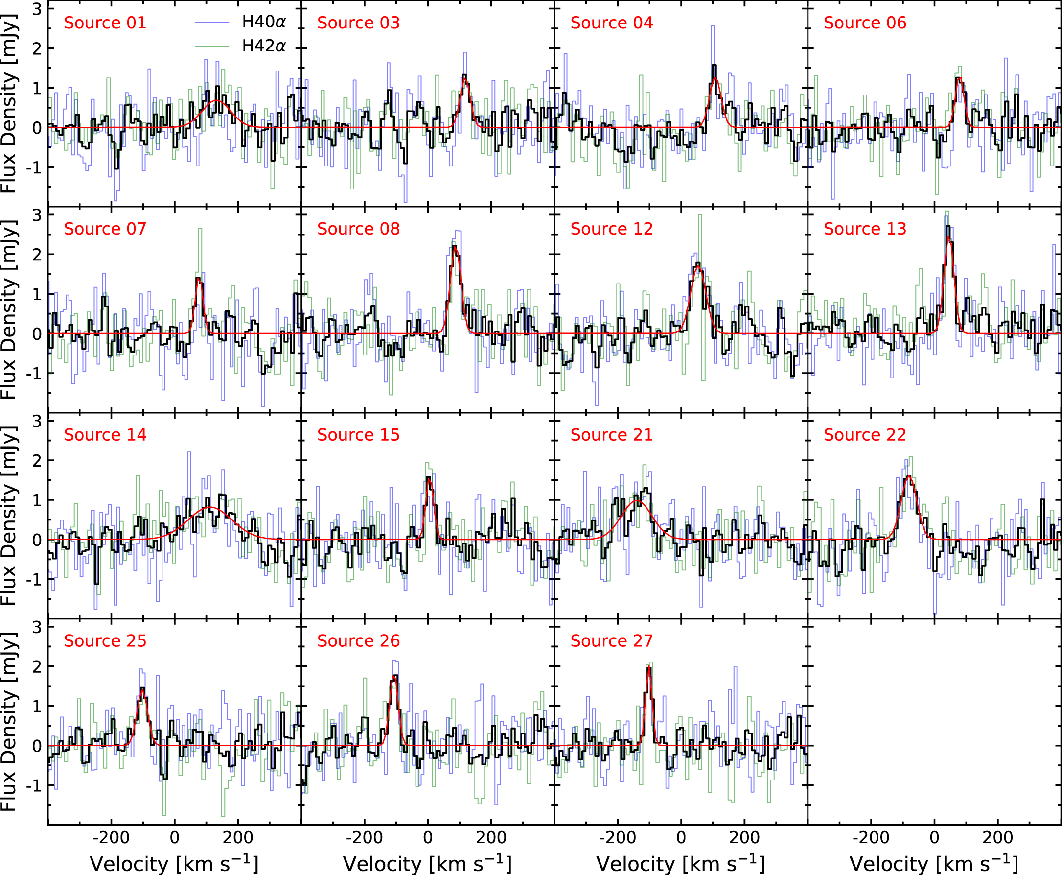
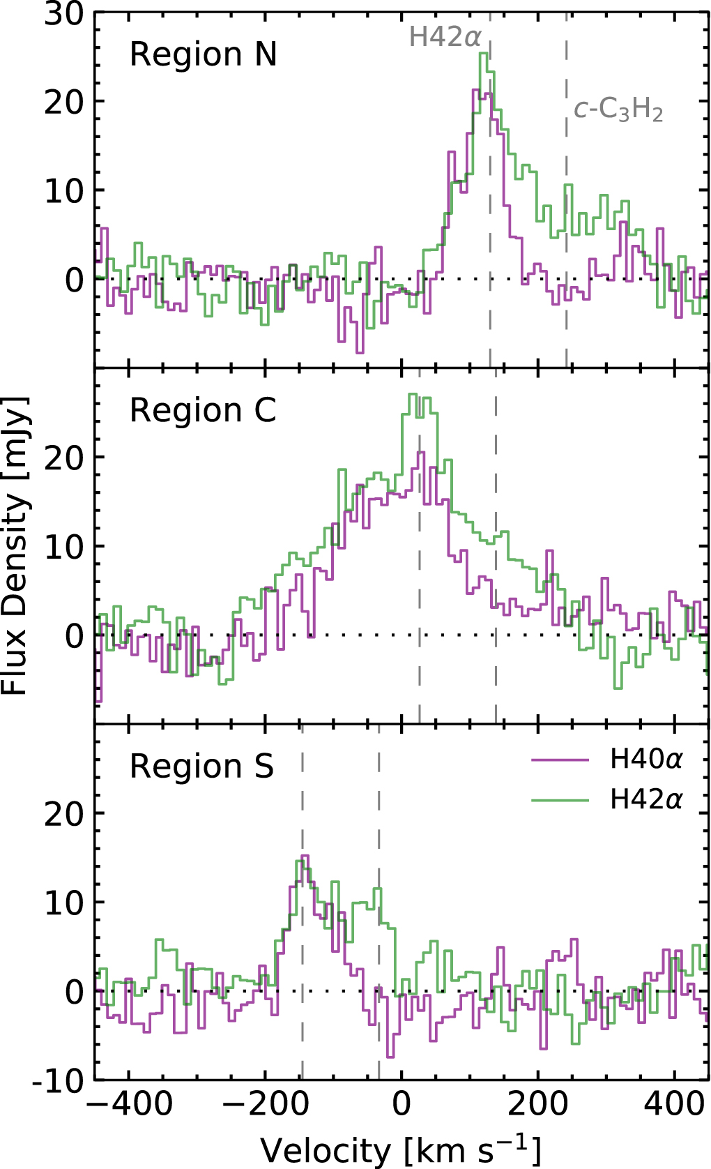