


Abstract
We present the hitherto largest sample of gas-phase metallicity radial gradients measured at sub-kpc resolution in star-forming galaxies in the redshift range of z ∈ [1.2, 2.3]. These measurements are enabled by the synergy of slitless spectroscopy from the Hubble Space Telescope near-infrared channels and the lensing magnification from foreground galaxy clusters. Our sample consists of 76 galaxies with stellar mass ranging from 107 to 1010  , an instantaneous star formation rate in the range of [1, 100]
  yr−1, and global metallicity
 ![$[\tfrac{1}{12},2]$](https://content.cld.iop.org/journals/0004-637X/900/2/183/revision1/apjabacceieqn3.gif) of solar. At a 2σ confidence level, 15/76 galaxies in our sample show negative radial gradients, whereas 7/76 show inverted gradients. Combining ours and all other metallicity gradients obtained at a similar resolution currently available in the literature, we measure a negative mass dependence of Δlog(O/H)/
of solar. At a 2σ confidence level, 15/76 galaxies in our sample show negative radial gradients, whereas 7/76 show inverted gradients. Combining ours and all other metallicity gradients obtained at a similar resolution currently available in the literature, we measure a negative mass dependence of Δlog(O/H)/![${\rm{\Delta }}r\,[\mathrm{dex}\,{\mathrm{kpc}}^{-1}]$](https://content.cld.iop.org/journals/0004-637X/900/2/183/revision1/apjabacceieqn4.gif) = (−0.020 ± 0.007) + (−0.016 ± 0.008)
= (−0.020 ± 0.007) + (−0.016 ± 0.008)  , with the intrinsic scatter being σ = 0.060 ± 0.006 over 4 orders of magnitude in stellar mass. Our result is consistent with strong feedback, not secular processes, being the primary governor of the chemostructural evolution of star-forming galaxies during the disk mass assembly at cosmic noon. We also find that the intrinsic scatter of metallicity gradients increases with decreasing stellar mass and increasing specific star formation rate. This increase in the intrinsic scatter is likely caused by the combined effect of cold-mode gas accretion and merger-induced starbursts, with the latter more predominant in the dwarf mass regime of
  .
.
Export citation and abstract BibTeX RIS
1. Introduction
Metallicity is one of the most fundamental proxies of galaxy evolution at the peak of cosmic star formation and metal enrichment (1 ≲ z ≲ 3), i.e., the cosmic noon epoch (Madau & Dickinson 2014). The interstellar medium oxygen abundance relative to hydrogen—metallicity12
—has been shown to correlate strongly with stellar mass ( ), star formation rate (SFR), and gas fraction (see the recent review by Maiolino & Mannucci 2019, and references therein). The cumulative history of the baryonic mass assembly, e.g., star formation, gas accretion, mergers, feedback, and galactic winds, altogether governs the total amount of metals remaining in gas (Finlator & Davé 2008; Davé et al. 2012; Lilly et al. 2013; Dekel & Mandelker 2014; Peng & Maiolino 2014). Moreover, these baryon cycling processes also tightly regulate the spatial distribution of metals in galaxies (Ho et al. 2015; Sanchez-Menguiano et al. 2016; Belfiore et al. 2019). Thus, a powerful way to learn about the baryon cycle is to use spatially resolved information.
The conventional way to obtain spatially resolved information is through integral field spectroscopy (IFS). This process has dramatically expanded our vision of galaxies from spectroscopic measurements integrated through single slits/fibers to panoramic two-dimensional (2D) views across their full surfaces, allowing for spatial variations of physical properties (including metallicity). This facilitates several large ground-based surveys (e.g., CALIFA, MaNGA, SAMI) to constrain the radial profile of metallicity in hundreds of galaxies, successfully capturing the dynamic signatures of the baryon cycle (see, e.g., Sanchez et al. 2014; Belfiore et al. 2017; Poetrodjojo et al. 2018). Meanwhile, numerical simulations are now capable of making useful predictions for metallicity radial gradients and their evolution with redshift (e.g., Ma et al. 2017; Tissera et al. 2019). The main challenge for observations is that sub-kpc spatial resolution is required for accurate results and meaningful comparison with theoretical predictions. While this spatial sampling is readily achieved for nearby galaxies (z ≲ 0.3), seeing-limited data are insufficient for galaxies at moderate to high redshift. Therefore, we need an effective approach to achieve sub-kpc resolved spectroscopy for statistically representative samples of high-z galaxies to compare meaningfully with cosmological zoom-in simulations.
The approach we take is space-based slitless spectroscopy. Building upon our previous efforts (Jones et al. 2015; Wang et al. 2017, 2019), we exploit grism spectroscopy from the Hubble Space Telescope (HST). The HST's diffraction limit in near-infrared wavelengths is equivalent to a physical scale of ∼1 kpc at z ∼ 2. Additional gains in resolution can be provided by gravitational lensing by foreground galaxies and/or galaxy clusters to fully satisfy the requirement for sufficiently resolving the chemical profiles of galaxies at that epoch. Lensing is thus essential for resolving the lowest-mass galaxies at high redshifts. Recently, Curti et al. (2020) derived metallicity maps and radial gradients in a sample of 28 lensed galaxies with stellar masses as low as 109  . In this work, we measure radial gradients of metallicity in 76 star-forming galaxies at 1.2 ≲ z ≲ 2.3 gravitationally lensed by foreground galaxy clusters, further extending to even lower stellar masses. Our sample enables a detailed comparison between observed and simulated chemostructural properties of galaxies, offering valuable insights into galaxy evolution.
This paper is organized as follows. In Section 2, we describe the data and galaxy sample analyzed in this work. The measurements of various physical quantities for our sample galaxies are presented in Section 3. Then, two major pieces of our analysis results, i.e., the redshift evolution and mass dependence of sub-kpc resolution metallicity gradients, are shown in Sections 4 and 5, respectively. We finally conclude in Section 6. Throughout this paper, the AB magnitude system and standard concordance cosmology ( = 0.3,
  = 0.7,
  ) are used. Forbidden lines are indicated as
 ![$[{\rm{O}}\,{\rm\small{III}}]$](https://content.cld.iop.org/journals/0004-637X/900/2/183/revision1/apjabacceieqn12.gif) λ5008 :=
λ5008 := ![$[{\rm{O}}\,{\rm\small{III}}]$](https://content.cld.iop.org/journals/0004-637X/900/2/183/revision1/apjabacceieqn13.gif) ,
, ![$[{\rm{O}}\,{\rm\small{II}}]$](https://content.cld.iop.org/journals/0004-637X/900/2/183/revision1/apjabacceieqn14.gif) λλ3727, 3730 :=
λλ3727, 3730 := ![$[{\rm{O}}\,{\rm\small{II}}]$](https://content.cld.iop.org/journals/0004-637X/900/2/183/revision1/apjabacceieqn15.gif) ,
, ![$[{\rm{N}}\,{\rm\small{II}}]$](https://content.cld.iop.org/journals/0004-637X/900/2/183/revision1/apjabacceieqn16.gif) λ6585 :=
λ6585 := ![$[{\rm{N}}\,{\rm\small{II}}]$](https://content.cld.iop.org/journals/0004-637X/900/2/183/revision1/apjabacceieqn17.gif) ,
, ![$[{\rm{S}}\,{\rm\small{II}}]$](https://content.cld.iop.org/journals/0004-637X/900/2/183/revision1/apjabacceieqn18.gif) λλ6718,6732 :=
λλ6718,6732 := ![$[{\rm{S}}\,{\rm\small{II}}]$](https://content.cld.iop.org/journals/0004-637X/900/2/183/revision1/apjabacceieqn19.gif) , if presented without wavelength values.
, if presented without wavelength values.
2. Data and Sample Selection
The spectroscopic data analyzed in this work are acquired by the Grism Lens-Amplified Survey from Space13
(GLASS; Proposal ID 13459, PI: Treu; Schmidt et al. 2014; Treu et al. 2015). It is a cycle 21 HST large program allocated 140 orbits of Wide-Field Camera 3 (WFC3) near-infrared slitless spectroscopy on the centers of 10 strong-lensing galaxy clusters. For each cluster center field, we have 10 orbits of G102 (covering 0.8–1.15  ) and four orbits of G141 (covering 1.1–1.7
  ) exposures, amounting to ∼22 ks of G102 and ∼9 ks of G141 in total, together with ∼7 ks of F105W+F140W direct imaging for wavelength/flux calibration and astrometric alignment. This exposure time is divided equally into two orients with almost orthogonal light dispersion directions, designed to disentangle contamination from neighbor objects. As a result, we obtain two suites of G102+G141 spectra for each object in an uninterrupted wavelength range of 0.8–1.7
  with nearly uniform sensitivity, reaching a 1σ surface brightness of 3 × 10⁻¹⁶
  . The 10 cluster fields are listed in Table 1 and shown in Figure 1. Among these clusters, six have ultradeep seven-filter imaging from the Hubble Frontier Fields (HFF) initiative (Lotz et al. 2017). The other four have multiband imaging from the Cluster Lensing And Supernova survey with Hubble (CLASH; Postman et al. 2012).

Figure 1. Color-composite images of the nine cluster center fields presented in this work (for the 10th field, i.e., MACS 1149, see Figure 1 of Wang et al. 2017). The blue, green, and red channels are stacked images from the HFF/CLASH mosaics taken at various filters, shown to the right of each panel. The footprints of HST WFC3 near-infrared grism pointings are denoted by the red and green squares, with the corresponding wavelength dispersion directions marked by the arrows in the same color in the upper right corner. The cyan contours represent the critical curves at the sample median redshift (z = 1.63) predicted by our default macroscopic lens models (see Section 3.6). Our sources with sub-kpc resolution metallicity gradient measurements are marked by magenta circles.
Download figure:
Standard image High-resolution imageTable 1. Summary of the HST Observations Presented in This Work
| Cluster Field | Cluster Alias | Cluster Redshift | R.A. | Decl. | Grism PAa | HST Imaging |
 b
b
|
|---|---|---|---|---|---|---|---|
| (deg) | (deg) | (deg) | |||||
| Abell 370 | A370 | 0.375 | 02:39:52.9 | −01:34:36.5 | 155, 253 | HFF | 7 |
| Abell 2744 | A2744 | 0.308 | 00:14:21.2 | −30:23:50.1 | 135, 233 | HFF | 13 |
| MACS 0416.1–2403 | MACS 0416 | 0.420 | 04:16:08.9 | −24:04:28.7 | 164, 247 | HFF/CLASH | 9 |
| MACS 0717.5+3745 | MACS 0717 | 0.548 | 07:17:34.0 | +37:44:49.0 | 020, 280 | HFF/CLASH | 5 |
| MACS 0744.9+3927 | MACS 0744 | 0.686 | 07:44:52.8 | +39:27:24.0 | 019, 104 | CLASH | 6 |
| MACS 1423.8+2404 | MACS 1423 | 0.545 | 14:23:48.3 | +24:04:47.0 | 008, 088 | CLASH | 9 |
| MACS 2129.4–0741 | MACS 2129 | 0.570 | 21:29:26.0 | −07:41:28.0 | 050, 328 | CLASH | 10 |
| RX J1347.5–1145 | RX J1347 | 0.451 | 13:47:30.6 | −11:45:10.0 | 203, 283 | CLASH | 2 |
| RX J2248.7–4431 | RX J2248 | 0.348 | 22:48:44.4 | −44:31:48.5 | 053, 133 | HFF/CLASH | 5 |
| MACS 1149.6+2223c | MACS 1149 | 0.544 | 11:49:36.3 | +22:23:58.1 | 032, 111, 119, 125 | HFF/CLASH | 10 |
Notes. Here we only list the primary pointings of the analyzed HST slitless spectroscopy covering the cluster centers with WFC3/NIR grisms.
aThe PAs are represented by the "PA_V3" values reported in the corresponding raw image headers. The PA of the actual dispersion axis of slitless spectroscopy, in degrees east of north, is given by . For each of the GLASS PAs (i.e., excluding PAs 111 and 119 for MACS 1149), two orbits of G141 and five orbits of G102 exposures have been taken, amounting to ∼4.5 and ∼11 ks science exposure times for G141 and G102, respectively.
bThe number of galaxies in which we secure sub-kpc resolution metallicity gradient measurements from HST spectroscopy.
cThe detailed analyses of gradient measurements have already been presented in our earlier paper (Wang et al. 2017). Here we update the SED fitting results associated with these galaxies.
. For each of the GLASS PAs (i.e., excluding PAs 111 and 119 for MACS 1149), two orbits of G141 and five orbits of G102 exposures have been taken, amounting to ∼4.5 and ∼11 ks science exposure times for G141 and G102, respectively.
bThe number of galaxies in which we secure sub-kpc resolution metallicity gradient measurements from HST spectroscopy.
cThe detailed analyses of gradient measurements have already been presented in our earlier paper (Wang et al. 2017). Here we update the SED fitting results associated with these galaxies.
Download table as: ASCIITypeset image
We base our source selection on the redshift catalogs made public by the GLASS collaboration. From these catalogs, we select 327 galaxies with secure spectroscopic redshifts in the range of z ∈ [1.2, 2.3] with the redshift quality flag ≥3. This redshift range is chosen to enable the grism coverage of the oxygen collisionally excited lines and the Balmer lines in the rest-frame optical (i.e., ![$[{\rm{O}}\,{\rm\small{III}}]$](https://content.cld.iop.org/journals/0004-637X/900/2/183/revision1/apjabacceieqn26.gif) , Hβ,
, Hβ, ![$[{\rm{O}}\,{\rm\small{II}}]$](https://content.cld.iop.org/journals/0004-637X/900/2/183/revision1/apjabacceieqn27.gif) ), which are the most promising and frequently used metallicity diagnostics at extragalactic distances. We also visually inspect the spatial extent and grism data quality of each source to remove sources with compact morphology (i.e., with half-light radius R50 <0
), which are the most promising and frequently used metallicity diagnostics at extragalactic distances. We also visually inspect the spatial extent and grism data quality of each source to remove sources with compact morphology (i.e., with half-light radius R50 <0 25 measured in
  -band imaging) and/or severe grism defects not suitable for our analysis. As a consequence, we compile a list of 93 objects with secure spectroscopic redshifts, relatively extended spatial profiles, and no severe defects or lack of data in their grism spectra. After further removing the sources with low signal-to-noise ratio (S/N) detections of emission lines (see Section 3.1) and ionization contamination from the active galactic nucleus (AGN; see Section 3.4), we obtain the final sample, comprising a total of 76 star-forming galaxies at z ∈ [1.2, 2.3], on which we present the subsequent measurements.
3. Methodology and Measurements
3.1. Emission Line Flux
We adopt the Grism Redshift and Line Analysis software (Grizli;14 G. Brammer et al. 2020, in preparation) to handle wide-field slitless spectroscopy data reduction. Grizli is state-of-the-art software that performs "one-stop shopping" processing of paired direct and grism exposures acquired by space telescopes. The entire procedure consists of five steps: (1) preprocessing raw grism exposures,15 (2) forward modeling full field-of-view (FoV) grism images, (3) redshift fitting via spectral template synthesis, (4) refining the full FoV grism model, and (5) extracting 1D/2D spectra and emission line maps of individual targets.
In step (3), we derive the best-fit redshift of our sources from spectral template fitting based on a library of spectral energy distributions (SEDs) of stellar populations with a range of characteristic ages (see Appendix A in Wang et al. 2019, for more details). We also fit the intrinsic nebular emission using 1D Gaussian functions centered at corresponding wavelengths and estimate the line fluxes. The morphological broadening is taken into account with respect to the dispersion direction associated with each exposure. Figure 2 shows the typical 1D and 2D spectra of one of our target galaxies. The majority (61/76) of our sample galaxies have ![$[{\rm{O}}\,{\rm\small{III}}]$](https://content.cld.iop.org/journals/0004-637X/900/2/183/revision1/apjabacceieqn29.gif) detected with S/N ≳ 10. Within the entire sample, 55, 35, and 15 have S/N ≳ 5 detections of
detected with S/N ≳ 10. Within the entire sample, 55, 35, and 15 have S/N ≳ 5 detections of ![$[{\rm{O}}\,{\rm\small{II}}]$](https://content.cld.iop.org/journals/0004-637X/900/2/183/revision1/apjabacceieqn30.gif) , Hβ, and Hγ, respectively. For galaxies at z ≤ 1.6, we also typically have access to their Hα16
and
, Hβ, and Hγ, respectively. For galaxies at z ≤ 1.6, we also typically have access to their Hα16
and ![$[{\rm{S}}\,{\rm\small{II}}]$](https://content.cld.iop.org/journals/0004-637X/900/2/183/revision1/apjabacceieqn31.gif) , which help constrain metallicity and nebular extinction. The best-fit redshifts and observed emission line fluxes for all of our sources are presented in Table A1.
, which help constrain metallicity and nebular extinction. The best-fit redshifts and observed emission line fluxes for all of our sources are presented in Table A1.

Figure 2. The HST grism spectra for one exemplary object in our sample, MACS 0416–ID 00955, at z ∼ 2. The total on-target exposure time is equally split between two nearly orthogonal PAs (shown in the two subfigures), reaching five orbits of G102 and two orbits of G141 exposures per PA. In each subfigure, we show the optimally extracted 1D spectra and the full 2D spectra with and without source stellar continuum subtraction for both grism channels. The 1D observed Fλ flux and its 1σ uncertainty are represented by the blue solid lines and cyan shaded bands, respectively. The wavelengths of the nebular line emission features are marked by magenta vertical dotted lines and red arrows in 1D and 2D spectra, respectively. The red dashed curves show the 1D model spectra, combining both stellar continuum (given by spectral template synthesis) and nebular line emission (modeled as Gaussian profiles), after the source morphological broadening is already taken into account. We emphasize that the same best-fit spectral model is used for each individual source, yet the differences in continuum shape and flux levels at the two PAs are originating from the varying source morphological kernels along the two light dispersion directions.
Download figure:
Standard image High-resolution image3.2. Emission Line Maps
In addition to the measurements of integrated emission line fluxes, another key piece of information that we need to retrieve from grism spectroscopy is the spatial distribution of emission line surface brightnesses, i.e., the emission line maps. The HST WFC3 near-infrared grisms have limited spectral resolution; for point sources, R ∼ 210 and 130 for G102 and G141, respectively. Yet this is actually an advantage in obtaining emission line maps. Since the instrument FWHM is equivalently ∼700 km s−1 for G102 and ∼1200 km s−1 for G141, it is reasonable to assume that the source 1D spectral shapes and 2D emission line maps are not affected by any kinematic motions of gas ionized by the star-forming regions, where outflows typically have speeds <500 km s−1 (see, e.g., Erb 2015, for a recent review). However, our sample galaxies are selected to be spatially extended, having their half-light radius R50 ≳ 025, measured from their continuum morphology in the  -band imaging acquired by HFF or CLASH. Their spatial profiles along the light dispersion direction are convolved onto the wavelength axis, resulting in severe morphological broadening of the line-spread function FWHM (van Dokkum et al. 2011). This morphological broadening effect is already taken into account when estimating the best-fit grism redshift from the spectral template synthesis process described in Section 3.1. It also poses a great challenge for obtaining spatial 2D maps of emission lines that have very close rest-frame wavelengths, in particular the line complex of Hβ +
 ![$[{\rm{O}}\,{\rm\small{III}}]$](https://content.cld.iop.org/journals/0004-637X/900/2/183/revision1/apjabacceieqn33.gif) λλ4960, 5008 doublets.
λλ4960, 5008 doublets.
We hence develop a custom technique to deblend the line complex as follows. First, we measure the source broadband isophotes that encompass over 90% of the surface brightness in the  and
and  bands and overlay them on the source 2D G141 and G102 spectra, respectively. The 2D grism spectra are standard data products produced by our Grizli reduction with contamination and source continuum removed. The positions of the overlaid isophotes on the 2D grism spectra mark the locations of the redshifted emission lines (see the middle and bottom rows of Figure 3). We rely on the preimaging (i.e.,
  and
and  ) paired with the grism (i.e., G141 and G102) observations to measure the isophotes because they cover a similar wavelength range, share comparable point-spread function (PSF) properties, and are acquired at the same position angle (PA) of the telescope. In this step, the grism spectra taken at different PAs have to be processed separately, since the morphological broadening varies drastically among different PAs if the source has asymmetric radial profiles. This broadband isophote is used as an aperture for emission line map extraction. Since the red (i.e., more to the right on the wavelength axis in 2D spectra) portion of the aperture centered at redshifted
 ![$[{\rm{O}}\,{\rm\small{III}}]$](https://content.cld.iop.org/journals/0004-637X/900/2/183/revision1/apjabacceieqn38.gif) λ5008 is not contaminated by
λ5008 is not contaminated by ![$[{\rm{O}}\,{\rm\small{III}}]$](https://content.cld.iop.org/journals/0004-637X/900/2/183/revision1/apjabacceieqn39.gif) λ4960, and the flux ratio between the
λ4960, and the flux ratio between the ![$[{\rm{O}}\,{\rm\small{III}}]$](https://content.cld.iop.org/journals/0004-637X/900/2/183/revision1/apjabacceieqn40.gif) doublets is fixed (
doublets is fixed (![${f}_{[{\rm{O}}{\rm\small{III}}]5008}/{f}_{[{\rm{O}}{\rm\small{III}}]4960}=2.98:1$](https://content.cld.iop.org/journals/0004-637X/900/2/183/revision1/apjabacceieqn41.gif) ; calculated by Storey & Zeippen 2000), we can obtain the same red portion of the clean
; calculated by Storey & Zeippen 2000), we can obtain the same red portion of the clean ![$[{\rm{O}}\,{\rm\small{III}}]$](https://content.cld.iop.org/journals/0004-637X/900/2/183/revision1/apjabacceieqn42.gif) λ4960 2D map. This red part of the
λ4960 2D map. This red part of the ![$[{\rm{O}}\,{\rm\small{III}}]$](https://content.cld.iop.org/journals/0004-637X/900/2/183/revision1/apjabacceieqn43.gif) λ4960 map is contaminating the slightly bluer part of the
λ4960 map is contaminating the slightly bluer part of the ![$[{\rm{O}}\,{\rm\small{III}}]$](https://content.cld.iop.org/journals/0004-637X/900/2/183/revision1/apjabacceieqn44.gif) λ5008 map and can be subtracted off, with flux errors properly propagated, therefore yielding cleaned
λ5008 map and can be subtracted off, with flux errors properly propagated, therefore yielding cleaned ![$[{\rm{O}}\,{\rm\small{III}}]$](https://content.cld.iop.org/journals/0004-637X/900/2/183/revision1/apjabacceieqn45.gif) λ5008 flux in those slightly bluer areas within the extraction aperture. This procedure is then conducted iteratively, until the
λ5008 flux in those slightly bluer areas within the extraction aperture. This procedure is then conducted iteratively, until the ![$[{\rm{O}}\,{\rm\small{III}}]$](https://content.cld.iop.org/journals/0004-637X/900/2/183/revision1/apjabacceieqn46.gif) λ4960 fluxes in all spatial pixels within the aperture have been removed and clean 2D maps of
λ4960 fluxes in all spatial pixels within the aperture have been removed and clean 2D maps of ![$[{\rm{O}}\,{\rm\small{III}}]$](https://content.cld.iop.org/journals/0004-637X/900/2/183/revision1/apjabacceieqn47.gif) λ5008 and Hβ can be obtained at individual PAs. Finally, we use AstroDrizzle (Gonzaga 2012) to combine the clean
λ5008 and Hβ can be obtained at individual PAs. Finally, we use AstroDrizzle (Gonzaga 2012) to combine the clean ![$[{\rm{O}}\,{\rm\small{III}}]$](https://content.cld.iop.org/journals/0004-637X/900/2/183/revision1/apjabacceieqn48.gif) λ5008 and Hβ maps extracted at multiple PAs. The resultant 2D stamps are drizzled onto a 006 grid, Nyquist sampling the FWHM of the WFC3 PSF, and astrometrically matched to the corresponding broadband images. Notably, our custom deblending technique does not rely on any models of the spatial profiles of
λ5008 and Hβ maps extracted at multiple PAs. The resultant 2D stamps are drizzled onto a 006 grid, Nyquist sampling the FWHM of the WFC3 PSF, and astrometrically matched to the corresponding broadband images. Notably, our custom deblending technique does not rely on any models of the spatial profiles of ![$[{\rm{O}}\,{\rm\small{III}}]$](https://content.cld.iop.org/journals/0004-637X/900/2/183/revision1/apjabacceieqn49.gif) emission.17
This is a critical procedure to account for the orient-specific contaminations of
emission.17
This is a critical procedure to account for the orient-specific contaminations of ![$[{\rm{O}}\,{\rm\small{III}}]$](https://content.cld.iop.org/journals/0004-637X/900/2/183/revision1/apjabacceieqn52.gif) λ4960, which can be over 2σ in some spatial areas within the extraction aperture (see the top right panel of Figure 3).
λ4960, which can be over 2σ in some spatial areas within the extraction aperture (see the top right panel of Figure 3).

Figure 3. Our custom technique of obtaining pure ![$[{\rm{O}}\,{\rm\small{III}}]$](https://content.cld.iop.org/journals/0004-637X/900/2/183/revision1/apjabacceieqn53.gif) λ5008 maps combined from multiple orients of grism exposures. Top, from left to right: color-composite image of object MACS 0416–ID 00955 (a z ∼ 2 dwarf galaxy with
λ5008 maps combined from multiple orients of grism exposures. Top, from left to right: color-composite image of object MACS 0416–ID 00955 (a z ∼ 2 dwarf galaxy with  ≃ 108
≃ 108  ), its
 ![$[{\rm{O}}\,{\rm\small{III}}]$](https://content.cld.iop.org/journals/0004-637X/900/2/183/revision1/apjabacceieqn56.gif) map before deblending the
map before deblending the ![$[{\rm{O}}\,{\rm\small{III}}]$](https://content.cld.iop.org/journals/0004-637X/900/2/183/revision1/apjabacceieqn57.gif) doublets, its pure
doublets, its pure ![$[{\rm{O}}\,{\rm\small{III}}]$](https://content.cld.iop.org/journals/0004-637X/900/2/183/revision1/apjabacceieqn58.gif) λ5008 map clean from the partial contamination of
λ5008 map clean from the partial contamination of ![$[{\rm{O}}\,{\rm\small{III}}]$](https://content.cld.iop.org/journals/0004-637X/900/2/183/revision1/apjabacceieqn59.gif) λ4960 at two orients (PA164 and PA247), and the significance of the difference between these two
λ4960 at two orients (PA164 and PA247), and the significance of the difference between these two ![$[{\rm{O}}\,{\rm\small{III}}]$](https://content.cld.iop.org/journals/0004-637X/900/2/183/revision1/apjabacceieqn60.gif) maps. The significance is expressed as the flux differences divided by the corresponding flux uncertainties (i.e., σ) of
maps. The significance is expressed as the flux differences divided by the corresponding flux uncertainties (i.e., σ) of ![$[{\rm{O}}\,{\rm\small{III}}]$](https://content.cld.iop.org/journals/0004-637X/900/2/183/revision1/apjabacceieqn61.gif) λ5008 in each spatial pixel. Middle and bottom: 2D contamination and continuum-subtracted G141 spectra of this dwarf galaxy at two orients (PA164 and PA274) separately. Note that these 2D traces are basically cutouts from the continuum-subtracted G141 spectra presented in Figure 2. Due to the limited spectral resolutions of HST grisms and extended source morphology, fluxes of
λ5008 in each spatial pixel. Middle and bottom: 2D contamination and continuum-subtracted G141 spectra of this dwarf galaxy at two orients (PA164 and PA274) separately. Note that these 2D traces are basically cutouts from the continuum-subtracted G141 spectra presented in Figure 2. Due to the limited spectral resolutions of HST grisms and extended source morphology, fluxes of ![$[{\rm{O}}\,{\rm\small{III}}]$](https://content.cld.iop.org/journals/0004-637X/900/2/183/revision1/apjabacceieqn62.gif) λ4960 are blended into
λ4960 are blended into ![$[{\rm{O}}\,{\rm\small{III}}]$](https://content.cld.iop.org/journals/0004-637X/900/2/183/revision1/apjabacceieqn63.gif) λ5008 and Hβ in a spatially inhomogeneous fashion, specific to the light dispersion direction at individual orients.
λ5008 and Hβ in a spatially inhomogeneous fashion, specific to the light dispersion direction at individual orients.
Download figure:
Standard image High-resolution image3.3. Stellar Mass
We perform SED fitting to the broadband photometry of our galaxies from the HST imaging data obtained by HFF or CLASH. The FAST software (Kriek et al. 2009) is used to infer stellar mass ( ), star formation rate (SFRS; see Section 3.5 for more details), and dust extinction of the stellar continuum (
 ) based on the Bruzual & Charlot (2003, hereafter BC03) stellar population synthesis models. We assume the Chabrier (2003) initial mass function, a constant star formation history, the Calzetti et al. (2000) extinction law, and fixed stellar metallicity being one-fifth solar. Since the majority of our galaxies show strong nebular emission in their rest-frame optical, we need to subtract their nebular emission from the corresponding broadband fluxes to estimate more accurately the level of stellar continuum. We convolve the best-fit Gaussian profiles for each emission line at the source redshift with the HST bandpass throughput to derive the nebular flux and then subtract it from the measured broadband photometry. In Table A1, we show the observed
  -band magnitude before this correction and the reduction factor, which is a ratio between the
  -band flux before and after correcting for nebular emission. We verify that this correction is essential for deriving reliable
  estimates for galaxies on the low-mass end (
 ); without this correction,
  can be overestimated by as much as 0.7 dex. We present the results of our stellar continuum SED fitting in Table A1. Thanks to lensing magnification, our sample extends significantly into the low-mass regime at high z, highly complementary to the targets from ground-based surveys (e.g., KMOS3D; Wuyts et al. 2016).
3.4. AGN Contamination
Before carrying out the metallicity inference on our sample, we check for contamination of AGN ionizations. In Figure 4, we rely on the mass-excitation diagram to exclude AGN candidates from our sample. The demarcation scheme (Juneau et al. 2014) aims to separate AGNs from star-forming galaxies based on the SDSS DR7 emission line galaxies at z ∼ 0. This scheme has been shown to reproduce the bivariate distributions seen in a number of high-redshift galaxy samples out to z ∼ 1.5 (Juneau et al. 2014). We therefore discard sources in our sample that are 2σ away from the star-forming region in the diagram, given the measurement uncertainties on  and
and ![$[{\rm{O}}\,{\rm\small{III}}]$](https://content.cld.iop.org/journals/0004-637X/900/2/183/revision1/apjabacceieqn72.gif) /Hβ. To examine possible redshift-dependent trends in future sections, we subdivide our sample into three bins: 37, 24, and 15 galaxies at z ∈ [1.2, 1.6], [1.6, 1.9], and [1.9, 2.3], respectively, marked by different symbols in Figure 4.
/Hβ. To examine possible redshift-dependent trends in future sections, we subdivide our sample into three bins: 37, 24, and 15 galaxies at z ∈ [1.2, 1.6], [1.6, 1.9], and [1.9, 2.3], respectively, marked by different symbols in Figure 4.

Figure 4. Mass-excitation diagram for our galaxies. The demarcation curves are from Juneau et al. (2014) based on the z ∼ 0 SDSS DR7 emission line sample; AGNs are located mainly above the red curve, star-forming galaxies are located below the green curve, and AGN/star-forming composites are in between. Our entire sample is separated into three redshift bins: z < 1.6 (37 sources), 1.6 ≤ z < 1.9 (24 sources), and z ≥ 1.9 (15 sources), color-coded in sSFR. We show that the majority of our sources are located below the green curve, where the possibility of being classified as AGNs is low (<10%).
Download figure:
Standard image High-resolution imageMoreover, Coil et al. (2015) found that a +0.75 dex shift in  of the demarcation curves is necessary to match the loci of AGNs and star-forming galaxies in the MOSDEF surveys at z ∼ 2.3 to account for the redshift evolution of the mass–metallicity relation (MZR). On part of the sample, we also obtained Hα gas kinematics from the ground-based Keck OSIRIS observations (Hirtenstein et al. 2019). The integrated measurement of
 ![${f}_{[{\rm{N}}{\rm\small{II}}]}/{f}_{{\rm{H}}\alpha }$](https://content.cld.iop.org/journals/0004-637X/900/2/183/revision1/apjabacceieqn74.gif) is typically ≲0.1 at a 3σ confidence level, indicative of star-forming regions with no significant AGN contamination. We thus verify that there is no sign of significant AGN ionization in our sample.
is typically ≲0.1 at a 3σ confidence level, indicative of star-forming regions with no significant AGN contamination. We thus verify that there is no sign of significant AGN ionization in our sample.
3.5. SFR
We have two methods for estimating the SFR. First of all, the SFR can be obtained from the stellar continuum SED fitting outlined in Section 3.3. This method is sensitive to the underlying assumptions of star formation history and stellar population synthesis models adopted in the fitting procedure. Hereafter, we refer to these measurements as SFRS.
Second, the SFR can be derived from nebular emission after correcting for dust attenuation. From our Bayesian inference method presented in Section 3.6, we obtain posterior probability distributions of the dereddened Hβ flux, which can be converted to the intrinsic Hα luminosity given a source redshift. As a consequence, the SFR (hereafter denoted as SFRN) can then be calculated following the widely used calibration (Kennicutt 1998), i.e.,

appropriate for the Chabrier (2003) initial mass function. Unlike the measurements from SED fitting, this method provides a proxy of instantaneous star-forming activities on a timescale of ∼10 Myr. This short timescale is relevant to probe the highly dynamic feedback processes that are effective in redistributing metals (see, e.g., Hopkins et al. 2014). Therefore, we quote the values of SFRN as our fiducial SFR measurements if not stated otherwise.
We note that for our low-z sample (37 galaxies at z ∈ [1.2, 1.6]), Hα is covered by the WFC3/G141 grism. However, due to the low spectral resolution, it is heavily blended with ![$[{\rm{N}}\,{\rm\small{II}}]$](https://content.cld.iop.org/journals/0004-637X/900/2/183/revision1/apjabacceieqn75.gif) . We hence rely on the empirical prescription of Faisst et al. (2018) to subtract the contribution of
. We hence rely on the empirical prescription of Faisst et al. (2018) to subtract the contribution of ![$[{\rm{N}}\,{\rm\small{II}}]$](https://content.cld.iop.org/journals/0004-637X/900/2/183/revision1/apjabacceieqn76.gif) fluxes from the measured Hα flux based on the stellar mass and redshift of our galaxies (see Table A1 for the calculated
fluxes from the measured Hα flux based on the stellar mass and redshift of our galaxies (see Table A1 for the calculated ![$[{\rm{N}}\,{\rm\small{II}}]$](https://content.cld.iop.org/journals/0004-637X/900/2/183/revision1/apjabacceieqn77.gif) /Hα flux ratios). This ensures a more reliable estimate of SFRN that is less impacted by dust than the Hβ-based measurements.
/Hα flux ratios). This ensures a more reliable estimate of SFRN that is less impacted by dust than the Hβ-based measurements.
In the left panel of Figure 5, we show the loci of our galaxies in the diagram of SFR versus  . By selecting lensed galaxies via their nebular emission line flux, our sample reaches an instantaneous SFR limit of ∼1
  yr−1 at z ∼ 2. In comparison to mass-complete samples (from, e.g., the KMOS3D survey; Wuyts et al. 2016) and galaxies from the star-forming main sequence (SFMS; Speagle et al. 2014; Whitaker et al. 2014), we push the exploration of star-forming galaxies at cosmic noon by 1–2 dex deeper into the low-mass regime. We also show the loci of the spectral stacks from the WFC3 Infrared Spectroscopic Parallel (WISP) Survey (Henry et al. 2013), very close to that of our galaxies given similar observing strategies. We gain over 1 dex in
  thanks to lensing magnification and the 14-orbit depth of the GLASS data in each field.

Figure 5. Global properties of our sample. Left: SFR as a function of  for galaxies at cosmic noon. Our galaxies are represented by the symbols following the scheme in Figure 4 corresponding to different z bins. However, the color-coding reflects the specific SFR derived from stellar continuum SED fitting after subtracting emission line fluxes (see Section 3.3). The loci of our galaxies are consistent with that of the WISP survey (Henry et al. 2013), if the SFR inferred from dust-corrected nebular emission is adopted. We also show that in terms of mass coverage, our sample is highly complementary to the ground-based mass-complete sample of KMOS3D, which can only probe down to
  at z ∼ 2. Right: MZRs for high-z galaxies. The symbols of our sample now have the same color-coding as in Figure 4. Our galaxies follow similar trends of the MZRs from the WISP survey and Maiolino et al. (2008). In the low-mass regime (
 ), our galaxies are more metal-enriched than the simple extensions of those MZRs. These metal-enriched galaxies also have higher sSFRs than the sample average.
Download figure:
Standard image High-resolution image3.6. Metallicity and Its Radial Gradient
Following our previous work (Wang et al. 2017, 2019), we adopt a forward-modeling Bayesian method to simultaneously infer metallicity ( ), nebular dust extinction (
 ), and dereddened Hβ flux (fHβ) based on observed emission line fluxes directly, as measured in Section 3.1. We use flat priors for
  and
and  in the ranges of [7.0, 9.3] and [0, 4], respectively, which are appropriate for the Maiolino et al. (2008) strong-line calibrations adopted in our inference. For fHβ, we use the Jeffreys prior in the range of [0, 1000] in units of
  . The Markov Chain Monte Carlo (MCMC) sampler Emcee is used to explore the parameter space, with the likelihood function defined as

Here  represents each of the available emission lines among the set of
 ![$[{\rm{O}}\,{\rm\small{II}}]$](https://content.cld.iop.org/journals/0004-637X/900/2/183/revision1/apjabacceieqn90.gif) , Hγ, Hβ,
, Hγ, Hβ, ![$[{\rm{O}}\,{\rm\small{III}}]$](https://content.cld.iop.org/journals/0004-637X/900/2/183/revision1/apjabacceieqn91.gif) , Hα, and
, Hα, and ![$[{\rm{S}}\,{\rm\small{II}}]$](https://content.cld.iop.org/journals/0004-637X/900/2/183/revision1/apjabacceieqn92.gif) , and
, and  and
and  denote the
  flux and its uncertainty, dereddened given a value of
  drawn from the MCMC sampling. The Cardelli et al. (1989) galactic extinction law with
  = 3.1 is adopted to correct for dust reddening, and Ri is the expected flux ratio between
  and Hβ, with
  being its intrinsic scatter. The content of Ri varies from strong-line diagnostic to Balmer decrement depending on the associated
  . In practice, if
  is one of the Balmer lines, Ri is given by
  and
and  , i.e., the Balmer decrement ratios assuming case B recombination under fiducial
  region situations. Instead, if
  is one of the oxygen collisionally excited lines, we take the strong-line flux ratios (i.e.,
 ![${f}_{[{\rm{O}}{\rm\small{III}}]}/{f}_{{\rm{H}}\beta }$](https://content.cld.iop.org/journals/0004-637X/900/2/183/revision1/apjabacceieqn106.gif) and
and ![${f}_{[{\rm{O}}{\rm\small{II}}]}/{f}_{{\rm{H}}\beta }$](https://content.cld.iop.org/journals/0004-637X/900/2/183/revision1/apjabacceieqn107.gif) ) calibrated by Maiolino et al. (2008) as Ri. Last, if
) calibrated by Maiolino et al. (2008) as Ri. Last, if  is
is ![$[{\rm{S}}\,{\rm\small{II}}]$](https://content.cld.iop.org/journals/0004-637X/900/2/183/revision1/apjabacceieqn109.gif) , we rely on our strong-line calibration of
, we rely on our strong-line calibration of ![$[{\rm{S}}\,{\rm\small{II}}]$](https://content.cld.iop.org/journals/0004-637X/900/2/183/revision1/apjabacceieqn110.gif) /Hα presented in Wang et al. (2017).
/Hα presented in Wang et al. (2017).
This forward-modeling approach is superior to converting emission line flux ratios (e.g., R23, O32) to metallicity because it properly takes into account any weak nebular emission that falls short of the detection limit and avoids double-counting information, as happens when combining multiple flux ratios that involve the same line. All sources in our sample have S/N ≳ 10 in at least one of the oxygen collisionally excited lines and/or Hα (if the source redshift is z ≲ 1.6), yet the Hβ detection is usually not as strong given its intrinsic faintness. By not calculating observed emission line flux ratios but forward modeling observed line fluxes directly, we avoid compromising the high-S/N detections of the bright ![$[{\rm{O}}\,{\rm\small{III}}]$](https://content.cld.iop.org/journals/0004-637X/900/2/183/revision1/apjabacceieqn111.gif) and
and ![$[{\rm{O}}\,{\rm\small{II}}]$](https://content.cld.iop.org/journals/0004-637X/900/2/183/revision1/apjabacceieqn112.gif) lines by the faint Hβ lines. As a result, our forward-modeling methodology improves our ability to infer an accurate metallicity based on high-S/N detections of strong nebular lines (i.e.,
lines by the faint Hβ lines. As a result, our forward-modeling methodology improves our ability to infer an accurate metallicity based on high-S/N detections of strong nebular lines (i.e., ![$[{\rm{O}}\,{\rm\small{III}}]$](https://content.cld.iop.org/journals/0004-637X/900/2/183/revision1/apjabacceieqn113.gif) and
and ![$[{\rm{O}}\,{\rm\small{II}}]$](https://content.cld.iop.org/journals/0004-637X/900/2/183/revision1/apjabacceieqn114.gif) ) and does not necessarily require high-S/N detections of faint emission lines. In the left panel of Figure 6, we show the joint constraints on (
) and does not necessarily require high-S/N detections of faint emission lines. In the left panel of Figure 6, we show the joint constraints on ( ,
,  , fHβ) derived from the observed integrated emission line fluxes for the exemplary object MACS 0416–ID 00955, whose 1D/2D spectra are shown in Figures 2 and 3. Together, we also simulate a scenario for this observation with much worse S/N detection of Hβ, i.e., artificially increasing the observed Hβ uncertainty by a factor of 10 while keeping other measurements unchanged. It is found that the resultant constraint on
  for this simulated scenario stays similar. This test demonstrates that our metallicity inference method can still ensure reasonable constraints on
  , even in cases where some emission lines, such as Hβ, are only marginally detected. In the right panel of Figure 6, we show the histograms of metallicity inferences (median values) given by our forward-modeling technique in all individual Voronoi cells from our entire galaxy sample. We divide all of these metallicity measurements in terms of the observed S/N of Hβ in the corresponding Voronoi cells. Regardless of the Hβ S/N, the three histograms all peak at
  ∼8.0, consistent with the integrated metallicity measurements from other work in similar ranges of redshift and mass (see, e.g., Figure 5 and Maiolino et al. 2008; Henry et al. 2013). From this test, we show that there is no systematic offset of the distribution of inferred metallicities among the three groups divided by Hβ S/N, and our metallicity estimates do not simply revert to the prior used in our Bayesian inference.

Figure 6. Rigorous constraint on metallicity from our forward-modeling Bayesian inference method. Left: marginalized 1D/2D constraints on metallicity ( ), nebular dust extinction (
 ), and dereddened Hβ flux (fHβ) based on the integrated emission line fluxes of object MACS 0416–ID 00955, presented in Table A1 (also see Figures 2 and 3). The parameter inference values shown at the top of each column are medians with 1σ uncertainties drawn from the [16th, 50th, 84th] percentiles, marked by the vertical dashed lines in the 1D histograms. Green corresponds to the inference from the actual observed emission line fluxes where Hβ is detected at S/N ∼ 11 (i.e.,
  ). Blue results are derived with the uncertainty of Hβ artificially increased by a factor of 10 (i.e., S/N ∼ 1.1), and other emission line flux measurements are unchanged. The comparison between the green and blue results shows that although the constraints on
  and fHβ are severely worsened by the decrease in S/N of Hβ, the inference on
  remains largely unchanged. This comparison thereby testifies that our forward-modeling Bayesian inference of metallicity does not require high-S/N detection of Hβ. Right: histograms of median metallicities measured using our forward-modeling method in all individual Voronoi cells from our entire galaxy sample. The distribution of metallicity measurements is divided into three groups corresponding to three different ranges of Hβ-observed S/N in the corresponding Voronoi cells. The horizontal dotted line shows the flat prior of
  ∈ [7.0, 9.3] used in our Bayesian inference. We demonstrate that the returned metallicity estimates do not simply revert to the prior, and there is no systematic offset in our metallicity inference, even in the low-S/N regime of Hβ.
Download figure:
Standard image High-resolution imageOur forward-modeling Bayesian inference is first performed on the integrated emission line fluxes measured for each galaxy to yield global metallicity. In the right panel of Figure 5, we show the MZR from our sample, color-coded by the specific SFR ( ) obtained from the aforementioned analyses. We also overlay the MZR from the WISP survey derived using the same strong-line calibrations (Henry et al. 2013). It is encouraging to see that the two MZRs follow similar trends due to similar source selection techniques and observing strategies. Notably, our galaxies at the extreme low-mass end (
 ) show both elevated metallicity and specific SFR (sSFR). This is consistent with the hypothesis that these low-mass systems are in the phase of early mass assembly with efficient metal enrichment and minimum dilution from pristine gas infall.
In addition to the integrated emission line fluxes, from the procedures described in Section 3.2, we also obtain 2D spatial distributions of emission line surface brightnesses. We utilize Voronoi tessellation as in Wang et al. (2019) to divide spatial bins with nearly uniform S/Ns of the strongest emission line available (usually ![$[{\rm{O}}\,{\rm\small{III}}]$](https://content.cld.iop.org/journals/0004-637X/900/2/183/revision1/apjabacceieqn128.gif) ). Our spatially resolved analysis based on Voronoi tessellation is superior to averaging the signals in radial annuli because of azimuthal variations (as large as 0.2 dex) in metallicity spatial distribution in nearby spiral galaxies (Berg et al. 2015; Ho et al. 2017). Our Bayesian inference is then executed in each of the Voronoi bins for all sources, yielding their metallicity maps at sub-kpc resolution.
). Our spatially resolved analysis based on Voronoi tessellation is superior to averaging the signals in radial annuli because of azimuthal variations (as large as 0.2 dex) in metallicity spatial distribution in nearby spiral galaxies (Berg et al. 2015; Ho et al. 2017). Our Bayesian inference is then executed in each of the Voronoi bins for all sources, yielding their metallicity maps at sub-kpc resolution.
To get the intrinsic deprojected galactocentric distance scale for each Voronoi bin, we conduct detailed reconstructions of the source-plane morphology of each galaxy in our sample. We first obtain a 2D map of the stellar surface density ( ; e.g., as shown in Figure 7) for each source through pixel-by-pixel SED fitting following the prescription described in Section 3.3. Then the pixels in this map are ray-traced back to their source-plane positions according to the deflection fields given by the macroscopic cluster lens models. For all HFF clusters, we use the Sharon & Johnson version 4corr models (Johnson et al. 2014). For the CLASH-only clusters, except RX J1347, we use the Zitrin PIEMD+eNFW version 2 model. For RX J1347, we use our own model built closely following the approach in Johnson et al. (2014). To this delensed 2D
  map, we fit a 2D elliptical Gaussian function to determine the galaxy's inclination, axis ratio, and major-axis orientation so that the source intrinsic morphology is recovered from lensing distortion.

Figure 7. A z ∼ 2 star-forming dwarf galaxy ( ≃ 108
≃ 108  ) with a negative metallicity radial gradient, similar to that measured in our Milky Way (i.e., −0.07 ± 0.01; Smartt & Rolleston 1997). We show this as an example of the analysis procedures applied to our entire sample. Top, from left to right: color-composite stamp (from the HFF imaging), stellar surface density (
 ) map (obtained from pixel-by-pixel SED fitting to HFF photometry), and surface brightness maps of emission lines
 ![$[{\rm{O}}\,{\rm\small{III}}]$](https://content.cld.iop.org/journals/0004-637X/900/2/183/revision1/apjabacceieqn134.gif) , Hβ,
, Hβ, ![$[{\rm{O}}\,{\rm\small{II}}]$](https://content.cld.iop.org/journals/0004-637X/900/2/183/revision1/apjabacceieqn135.gif) , and Hγ. We use the technique demonstrated in Figure 3 to obtain pure
, and Hγ. We use the technique demonstrated in Figure 3 to obtain pure ![$[{\rm{O}}\,{\rm\small{III}}]$](https://content.cld.iop.org/journals/0004-637X/900/2/183/revision1/apjabacceieqn136.gif) λ5008 and Hβ maps for the source. The black contours mark the delensed, deprojected galactocentric radii with 1 kpc intervals given by our source-plane morphological reconstruction described in Section 3.6. Bottom: metallicity map and radial gradient determination for this galaxy. The weighted Voronoi tessellation technique (Cappellari & Copin 2003; Diehl & Statler 2006) is adopted to divide the surface into spatial bins with a constant S/N of 5 on
λ5008 and Hβ maps for the source. The black contours mark the delensed, deprojected galactocentric radii with 1 kpc intervals given by our source-plane morphological reconstruction described in Section 3.6. Bottom: metallicity map and radial gradient determination for this galaxy. The weighted Voronoi tessellation technique (Cappellari & Copin 2003; Diehl & Statler 2006) is adopted to divide the surface into spatial bins with a constant S/N of 5 on ![$[{\rm{O}}\,{\rm\small{III}}]$](https://content.cld.iop.org/journals/0004-637X/900/2/183/revision1/apjabacceieqn137.gif) . In the right panel, the metallicity measurements in these Voronoi bins are plotted as magenta points. The dashed magenta line denotes the linear regression, with the corresponding slope shown at the bottom. The spatial extent and orientation remain unchanged throughout all of the 2D maps in both rows, with north up and east to the left.
. In the right panel, the metallicity measurements in these Voronoi bins are plotted as magenta points. The dashed magenta line denotes the linear regression, with the corresponding slope shown at the bottom. The spatial extent and orientation remain unchanged throughout all of the 2D maps in both rows, with north up and east to the left.
Download figure:
Standard image High-resolution imageSince we have measured both metallicity and source-plane deprojected galactocentric radius for each Voronoi bin, we can estimate a radial gradient slope via linear regression (see Appendix A for the gradient measurements based on metallicities derived in source-plane Voronoi bins and related discussions about the effect of anisotropic lensing distortion). Figure 7 demonstrates the entire process for measuring the metallicity radial gradient of a z ∼ 2 star-forming dwarf galaxy. As a sanity check, we also measure its radial gradient using metallicity inferences derived in each individual spatial pixel and radial annulus. We verified that the differences among the three methods are ≲0.03 dex kpc−1, within the measurement uncertainties.
In the end, we secure a total of 76 galaxies in the redshift range of 1.2 ≲ z ≲ 2.3 with sub-kpc resolution metallicity gradients (see Table 1 for the number of sources in individual cluster center fields). This is hitherto the largest sample of such measurements in the distant universe. This sample enables robust measures of both average gradient slopes and scatter in the population.
4. The Cosmic Evolution of Metallicity Gradients at High Redshifts
In this section, we collect published results on radial gradients of metallicity measured in the distant universe. We focus on the measurements that are derived with sub-kpc resolution because insufficient spatial sampling is shown to cause spuriously flat gradient measurements (Yuan et al. 2013). This poses a real challenge for ground-based observations, given that the optimal seeing condition is ∼06, equivalent to 5 kpc at z ∼ 2. There have been a number of attempts to overcome this beam smearing through correcting the distorted light wave front with the adaptive optics (AO) technique. Using the SINFONI instrument on the Very Large Telescope under the AO mode, Swinbank et al. (2012) measured seven gradients at z ∼ 1.5. Following the same strategy, Förster Schreiber et al. (2018) expanded the sample by adding 21 new measurements at z ∼ 2 from the SINS/zC-SINF survey.18
Lensing can also help increase the spatial sampling rate. Jones et al. (2010, 2013) brought forward this approach by securing four gradients at z ∼ 2 in galaxy–galaxy lensing systems using the AO-assisted OSIRIS instrument on the Keck telescope, with resolution further boosted ≳3× by lensing magnification. Leethochawalit et al. (2016) carried out similar analyses and measured 11 new gradients at similar redshifts. To recap, there existed a total of 43 metallicity gradient measurements with sub-kpc spatial resolution at cosmic noon before our work.
In this work, we triple the sample size by presenting 76 sub-kpc resolution metallicity radial gradients in star-forming galaxies at cosmic noon. This is by far the largest homogeneous sample with sufficient spatial resolution, which enables a uniform analysis. In Figure 8, our results are highlighted by three sets of symbols—corresponding to the three z subgroups—color-coded in sSFR. From a total of 76 galaxies in our sample with sub-kpc resolution gradient measurements, there are 15 and seven sources showing negative and positive (i.e., inverted) gradients greater than 2σ away from being flat, respectively. At a 3σ confidence level, the number of galaxies showing negative and inverted gradients is seven and three, respectively. Notably, two of the three inverted gradients (A370–ID 03751 and MACS 0744–ID 01203) have already been reported in detail in Wang et al. (2019). All individual ground-based measurements at similar resolution (≲kpc scale) are represented by magenta squares. Recently, Curti et al. (2020) analyzed the KMOS observations in the field of RX J2248 and measured metallicity gradients in 12 background galaxies lensed by RX J2248, of which three are in overlap with our sample (i.e., ID 00206, ID 00428, and ID 01205). We verified that the gradient results measured from both works are compatible at a 1σ confidence level. It is encouraging to see that the metallicity gradients derived using different methods and data sets are in good agreement.

Figure 8. Overview of metallicity gradients in the distant universe. Our measurements are represented by three symbols, corresponding to different z ranges as in Figure 4, color-coded in sSFR. As a comparison, we also include individual measurements at similar resolution (≲kpc scale) from ground-based AO-assisted observations, marked by magenta squares (Swinbank et al. 2012; Jones et al. 2013; Leethochawalit et al. 2016; Förster Schreiber et al. 2018). The 2σ spreads of measurements from KMOS3D (Wuyts et al. 2016) and MUSE (Carton et al. 2018) and the simulation results from FIRE (Ma et al. 2017) are shown as shaded regions in green, yellow, and gray, respectively. The evolutionary tracks of two simulated disk galaxies (Milky Way analogs at z ∼ 0) with different feedback strengths but otherwise identical numerical setups are denoted by the two orange curves.
Download figure:
Standard image High-resolution imageSome theoretical trends are overlaid in Figure 8. In particular, two numerical simulations with different galactic feedback strengths but otherwise identical settings by Gibson et al. (2013) are shown as orange curves. The comparison between these two trends demonstrates that enhanced feedback can be highly efficient in erasing metal inhomogeneity. Therefore, resolved chemical properties, if measured accurately, can shed light on the strength of galactic feedback in the early phase of disk growth.
Figure 8 also shows the spread of the KMOS3D gradient measurements by Wuyts et al. (2016), which is highly clustered to flatness. Without AO support or lensing magnification gain on the spatial sampling rate, these gradients are usually obtained at an FWHM angular resolution of ∼06, imposed by the natural seeing. For a z ∼ 1.5 star-forming galaxy with intrinsically negative metallicity gradient (![${\rm{\Delta }}\mathrm{log}({\rm{O}}/{\rm{H}})/{\rm{\Delta }}r\,=-0.16\pm 0.02\,[\mathrm{dex}\,{\mathrm{kpc}}^{-1}]$](https://content.cld.iop.org/journals/0004-637X/900/2/183/revision1/apjabacceieqn139.gif) ), Yuan et al. (2013) showed that from seeing-limited observations with an FWHM angular scale of ∼05, its radial metallicity gradient is instead measured to be
), Yuan et al. (2013) showed that from seeing-limited observations with an FWHM angular scale of ∼05, its radial metallicity gradient is instead measured to be ![${\rm{\Delta }}\mathrm{log}({\rm{O}}/{\rm{H}})/{\rm{\Delta }}r=-0.01\pm 0.03\,[\mathrm{dex}\,{\mathrm{kpc}}^{-1}]$](https://content.cld.iop.org/journals/0004-637X/900/2/183/revision1/apjabacceieqn140.gif) , significantly biased toward flatness caused by beam smearing. To mitigate the potential bias from beam smearing, Carton et al. (2018) conducted a forward-modeling analysis to recover 65 gradients at 0.1 ≲ z ≲ 0.8 from the seeing-limited MUSE observations (marked in green in Figure 8).
, significantly biased toward flatness caused by beam smearing. To mitigate the potential bias from beam smearing, Carton et al. (2018) conducted a forward-modeling analysis to recover 65 gradients at 0.1 ≲ z ≲ 0.8 from the seeing-limited MUSE observations (marked in green in Figure 8).
The 2σ interval of the FIRE simulations (Ma et al. 2017) is shown as the gray shaded region in Figure 8. We see that the scatter predicted by the FIRE simulations matches well that from low-z observations (at z ≲ 1; e.g., from Carton et al. 2018), but it is smaller by a factor of 2 at higher redshifts, especially at z ≳ 1.3. This likely reflects that galaxies display more diverse chemostructural properties at the peak epoch of cosmic structure formation and metal enrichment, when star formation is more episodic and vigorous (see, e.g., Hopkins et al. 2014).
5. The Mass Dependence of Metallicity Gradients at sub-kpc Resolution: Testing Theories over 4 dex of M⋆
With the sample statistics greatly improved, we can quantify the mass dependence of reliably measured metallicity gradients at high redshifts as a test of theoretical predictions. The combined sample includes our 76 measurements at z ∈ [1.2, 2.3] and 3519
others, as given in Section 4. Following the same color/marker styles as in Figure 8, we plot these high-resolution gradient measurements as a function of their associated  in Figure 9. It is remarkable that now the observational data cover 4 orders of magnitude in
  . Notably, over half of our gradient measurements reside in the dwarf mass regime (
 ), probing ≳2 dex deeper into the low-mass end compared with the ground-based AO results (magenta squares).

Figure 9. Metallicity gradient as a function of stellar mass for high-z and local star-forming galaxies. As in Figure 8, our measurements are represented by three types of symbols regarding three z bins colored-coded in sSFR, whereas high-z ground-based measurements with similar resolution are denoted by magenta squares. For comparison, we also show the median measurements with a 1σ interval of local measurements (Belfiore et al. 2017; Bresolin 2019), the 2σ spread of the FIRE simulations (Ma et al. 2017), and two mass dependencies derived from the EAGLE simulations assuming different feedback settings (Tissera et al. 2019). Combining all available high-z gradients measured at sufficient spatial resolution (≲kpc), we obtain a weakly negative mass dependence over 4 orders of magnitude in  , Δlog(O/H)/
![${\rm{\Delta }}r\,[\mathrm{dex}\,{\mathrm{kpc}}^{-1}]$](https://content.cld.iop.org/journals/0004-637X/900/2/183/revision1/apjabacceieqn146.gif) = (−0.020 ± 0.007) + (−0.014 ± 0.008)
= (−0.020 ± 0.007) + (−0.014 ± 0.008)  , with the intrinsic scatter being σ = 0.060 ± 0.006. The thin tan lines mark 100 random draws from the linear regression. This observed mass dependence is in remarkable agreement with the predictions of the FIRE simulations. However, as shown in Table 2, we also observe an increase of the intrinsic scatter from high- to low-mass systems not captured by theoretical predictions.
Download figure:
Standard image High-resolution imageWe perform linear regression on all of these measurements of metallicity gradient and stellar mass, with errors on both quantities taken into account, using the following formula:

Here α and β are the intercept and slope of the linear function, respectively;  represents a normal distribution, with σ being the intrinsic scatter in units of
  ; and Mmed is the median of the input stellar masses taken as normalization. For the entire mass range (where
  ), we obtain the following estimates: α = −0.020 ± 0.007, β = −0.016 ± 0.008, and σ = 0.060 ± 0.006 (see the result of case I in Table 2). This shows a weak negative correction between metallicity gradient and stellar mass for these 111 high-z star-forming galaxies.
Table 2. Linear Regression Results of the Mass Dependence of Metallicity Radial Gradients at Cosmic Noon
| Case | α | β | σ |

|

|
Notes |
|---|---|---|---|---|---|---|
| I |

|

|

|

|
111 | All metallicity gradients measured at sub-kpc resolution |
| II |

|

|

|

|
76 | All metallicity gradients from HST spectroscopy |
| IIIa |

|

|

|

|
27 | High-mass bin: 
|
| IIIb |

|

|

|

|
47 | Medium-mass bin: 
|
| IIIc |

|

|

|

|
31 | Low-mass bin: 
|
| IVa |

|

|

|

|
50 | High-sSFR bin: 
|
| IVb |

|

|

|

|
61 | Low-sSFR bin: 
|
Note. The linear regression is performed using the linmix software (https://github.com/jmeyers314/linmix), taking into account the measurement uncertainties on both stellar mass ( ) and metallicity gradient (
 ), following the Bayesian method proposed by Kelly (2007). The following function form (Equation (3)) is adopted: Δlog(O/H)/
![${\rm{\Delta }}r\,[\mathrm{dex}\,{\mathrm{kpc}}^{-1}]=\alpha +\beta \mathrm{log}({M}_{* }/{M}_{\mathrm{med}})+N(0,{\sigma }^{2})$](https://content.cld.iop.org/journals/0004-637X/900/2/183/revision1/apjabacceieqn188.gif) . As given in the seventh column, case I corresponds to the linear regression result based on all sub-kpc-scale metallicity gradient measurements at the cosmic noon epoch, whereas case II shows the results from our gradient measurements only. We divide the entire sample into three
. As given in the seventh column, case I corresponds to the linear regression result based on all sub-kpc-scale metallicity gradient measurements at the cosmic noon epoch, whereas case II shows the results from our gradient measurements only. We divide the entire sample into three  bins and conduct linear regressions separately, with results represented by cases IIIa, b, and c. Cases IVa and b show the results if the entire sample is divided based on sSFR, instead of
  . The number of sources (
 ) involved in each case is shown in the sixth column.
Download table as: ASCIITypeset image
To understand this negative mass dependence, we show two theoretical predictions from the EAGLE simulations in Figure 9, corresponding to two suites of numerical simulations implementing different strengths of supernova feedback (Tissera et al. 2019). We see a drastic difference in the slope of the mass dependence of metallicity gradients predicted by different feedback settings in EAGLE, albeit the short  coverage. This difference is largely caused by the bifurcations seen in the temporal evolution of radial chemical profiles for individual galaxies, exemplified by the two simulation tracks shown in Figure 8. Under the assumption of weak feedback, galaxies evolve according to secular processes, and their radial gradients flatten over time (Pilkington et al. 2012). Given the mass assembly downsizing, more massive galaxies are in a later phase of disk growth than less massive ones (Brinchmann et al. 2004). Collectively, a positive mass dependence of radial gradients manifests. However, when feedback is enhanced, feedback-driven gas flows can efficiently mix stellar nucleosynthesis yields and prevent any metal inhomogeneity from emerging (Ma et al. 2017). This effect is more pronounced in lower-mass galaxies living in smaller dark matter halos with shallower gravitational potentials. As a result, a generally negative mass dependence (flat/inverted gradients at the low-mass end and negative gradients at the high-mass end) can be anticipated.
Figure 9 also shows the 2σ spread of the mass dependence from the FIRE simulations (Ma et al. 2017). Given the relatively strong feedback scheme implemented in FIRE, we expect a negative mass dependence, which is indeed seen. Remarkably, the predictions of the FIRE simulations match very well the linear regression fit based on the combined high-z metallicity gradient sample. Our result is thus in better agreement with enhanced feedback—rather than secular processes—playing a significant role in shaping the chemical enrichment and structural evolution during the disk mass assembly (Hopkins et al. 2014; Vogelsberger et al. 2014).
To verify that the observed trends are robust, we subdivide the gradient measurements into three mass bins and perform a separate linear regression analysis to each bin. The results are given in Table 2. We see that the intercept value becomes more negative as  increases, with the slopes all consistent with zero, confirming the negative mass dependence of metallicity gradients over the entire mass range. More importantly, we observe an increase in the intrinsic scatter of metallicity gradients with
  from high- to low-mass regimes, consistent with the findings in local spiral galaxies by Bresolin (2019). This increase in scatter can also be found if separating the galaxies based on their sSFR.20
For galaxies in the combined sample with
from high- to low-mass regimes, consistent with the findings in local spiral galaxies by Bresolin (2019). This increase in scatter can also be found if separating the galaxies based on their sSFR.20
For galaxies in the combined sample with  , the scatter is constrained to be
  (case IVa in Table 2), whereas for galaxies with sSFR ≲ 5 Gyr−1, the scatter is instead
  (case IVb in Table 2).
The increase of sSFR in low-mass systems can be ascribed to the accretion of low-metallicity gas from the cosmic filaments (i.e., cold-mode gas accretion; Dekel et al. 2009) or gravitational interaction events amplifying the star formation efficiency (i.e., merger-induced starbursts; Stott et al. 2013). Both of them can bring about large dispersions in the radial chemical profiles. To investigate which of the two effects is more dominant in boosting the chemostructural diversity in low-mass high-sSFR galaxies, we turn to the global MZR of our sample, presented in Section 3.6 (see Figure 5). We rely on the WISP measurements as the control sample because of the similar source selection criteria, mass coverage, redshift range, and consistent techniques in estimating SFR (based on Balmer line fluxes) and metallicity (assuming the Maiolino et al. 2008 calibrations).
We find that in the medium-mass bin (![${M}_{* }/{M}_{\odot }\,\in [{10}^{9},{10}^{10}]$](https://content.cld.iop.org/journals/0004-637X/900/2/183/revision1/apjabacceieqn198.gif) ), the galaxies in our sample with a higher SFR than that of the WISP stacks are more metal-poor by 0.15 dex than the WISP metallicities in the corresponding mass range. This is supportive of the cold-mode accretion diluting the global metallicity of our galaxies, stimulating star formation and increasing the intrinsic scatter of metallicity gradients. However, in the low-mass bin (
), the galaxies in our sample with a higher SFR than that of the WISP stacks are more metal-poor by 0.15 dex than the WISP metallicities in the corresponding mass range. This is supportive of the cold-mode accretion diluting the global metallicity of our galaxies, stimulating star formation and increasing the intrinsic scatter of metallicity gradients. However, in the low-mass bin (![${M}_{* }/{M}_{\odot }\in [{10}^{8},{10}^{9}]$](https://content.cld.iop.org/journals/0004-637X/900/2/183/revision1/apjabacceieqn199.gif) ), our galaxies with a higher SFR than WISP show significant metal enrichment, i.e., higher by 0.27 dex than the corresponding WISP metallicities. We hence argue that in the dwarf mass regime of
), our galaxies with a higher SFR than WISP show significant metal enrichment, i.e., higher by 0.27 dex than the corresponding WISP metallicities. We hence argue that in the dwarf mass regime of  , merger-driven starbursts play a more predominant role than the cold-mode accretion does to boost the chemostructural diversity. Our result is consistent with the sharp increase of the merger fraction—from 10% to over 50% for galaxies at
  –108.5 at z ∼ 1.5—found by the HiZELS survey (Stott et al. 2013, 2014). For the part of our dwarf galaxies on which we have mapped their gas kinematics using Keck OSIRIS, we also found that the velocity field becomes more turbulent (i.e., with lower ratios of rotational speed versus velocity dispersion) for galaxies with higher sSFR (Hirtenstein et al. 2019). This kinematic evidence further reinforces the scenario that mergers boost the star formation efficiency, random motions, and chemostructural diversity in dwarf galaxies at cosmic noon.
Lastly, the combined high-z metallicity gradient sample reveals that inverted gradients are almost exclusively found in the low-mass range, i.e.,  (see also Carton et al. 2018). This feature is also seen in the local universe; only the lowest
  bin (at
  ) from the MaNGA survey shows a positive gradient slope (Belfiore et al. 2017). The reason for inverted gradients in isolated systems is still under debate, with possible causes ranging from centrally directed cold-mode accretion (Cresci et al. 2010) to metal-loaded outflows triggered by galactic winds (Wang et al. 2019). In any case, these processes should be more pronounced in low-mass systems, suggested by the occurrence rate of this inverted-gradient phenomenon.
6. Conclusion
To summarize, we have presented an unprecedentedly large sample of sub-kpc resolution metallicity radial gradients in 76 gravitationally lensed star-forming galaxies at 1.2 ≲ z ≲ 2.3 using HST near-infrared slitless spectroscopy. We performed state-of-the-art reduction of grism data, careful stellar continuum SED fitting after subtracting nebular emission from broadband photometry, and Bayesian inferences of metallicity and SFR based on emission line fluxes. Our sample spans an  range of [107, 1010]
  , an instantaneous SFR range of [1, 100]
  yr−1, and a global metallicity range of 7.6 ≲
  ≲ 9.0, i.e.,
  , 2] solar. At a 2σ confidence level, we secured 15 and seven galaxies that show negative and inverted gradients, respectively. Collecting all high-resolution gradient measurements at high redshifts currently existing (where the results presented in this work constitute 2/3 of all measurements), we measure a weak negative mass dependence over 4 orders of magnitude in
  : Δlog(O/H)/
![${\rm{\Delta }}r\,[\mathrm{dex}\,{\mathrm{kpc}}^{-1}]$](https://content.cld.iop.org/journals/0004-637X/900/2/183/revision1/apjabacceieqn211.gif) = (−0.020 ± 0.007) + (−0.016 ± 0.008)
= (−0.020 ± 0.007) + (−0.016 ± 0.008)  , with σ = 0.060 ± 0.006 being the intrinsic scatter. This supports enhanced feedback as the main driver of the chemostructural evolution of star-forming galaxies at cosmic noon. Moreover, we also find that the intrinsic scatter of metallicity gradients increases with decreasing
  and increasing sSFR. Combined with the global metallicity measurements, our result is consistent with the hypothesis that the combined effect of cold-mode gas accretion and merger-induced starbursts strongly boosts the chemostructural diversity of low-mass star-forming galaxies at cosmic noon, with mergers playing a much more predominant role in the dwarf mass regime of
  . This work demonstrates that by accurately mapping the radial chemical profiles of star-forming galaxies at high redshifts, we can cast strong constraints on the role that feedback, gas flows, and mergers play in the early phase of disk mass assembly. The observed trends between metallicity and galaxy properties, while weak, are nonetheless very well measured over a wide dynamic range of mass. This census offers a stringent test for theoretical models and cosmological simulations, as the resulting trends are highly sensitive to baryon cycling processes at the peak of cosmic star formation (1.2 ≲ z ≲ 2.3). Using the Near-Infrared Imager and Slitless Spectrograph (NIRISS) on board the soon-to-be-launched James Webb Space Telescope (JWST), the GLASS-JWST ERS program (PI: Treu; ID 1324) and the CAnadian NIRISS Unbiased Cluster Survey (CANUCS) GTO program (PI: Willott) will conduct K-band slitless spectroscopy on several galaxy cluster center fields. The data acquired by these programs will enable sub-kpc resolution measurements of metallicity gradients to z ≲ 3.5 and thus extend the test for theoretical predictions to even higher redshifts.
We thank the anonymous referee for careful reading and constructive comments that improved the quality of our paper. This work is supported by NASA through HST grant HST-GO-13459. X.W. acknowledges support by UCLA through a dissertation year fellowship. X.W. is greatly indebted to his family, i.e., Dr. Xiaolei Meng, SX Wang, and ST Wang, for their tremendous love, care, and support during the COVID-19 pandemic, without which this work could not have been completed.
Software: APLpy (Robitaille & Bressert 2012), AstroDrizzle (Gonzaga 2012), Astropy (Price-Whelan et al. 2018), Emcee (Foreman-Mackey et al. 2013), FAST (Kriek et al. 2009), Grizli (G. Brammer et al. 2020, in preparation), SExtractor (Bertin & Arnouts 1996), VorBin (Cappellari & Copin 2003).
Appendix A: Measuring Metallicity Radial Gradients Using Voronoi Tessellation in the Source Plane
As explained in Section 3.6, we use Voronoi tessellation to divide the spatial extent of our sample galaxies into subregions, where we measure metallicities individually to estimate their radial gradients. This tessellation process is by default performed in the image plane, since the noise properties of the observed emission line fluxes are well defined in the image plane. Furthermore, the majority of our sample galaxies have magnifications less than 4, and the sample median value is μ = 2.69 (see the results presented in Table A1), which indicates that the highly anisotropic lensing phenomenon is relatively rare in our sample.
Table A1. Measured Quantities of Our Sample Galaxies
| Cluster | ID | R.A. | Decl. |

|

|
F140Wa |
 b
b
|
Observed Integrated Emission Line Fluxes   ) ) |
μc | Stellar Continuum SED Fitting | [N ii]/Hαd | Nebular Emission Diagnostics | |||||||||
|---|---|---|---|---|---|---|---|---|---|---|---|---|---|---|---|---|---|---|---|---|---|
| (deg) | (deg) | (dex kpc−1) | (AB mag) | ||||||||||||||||||
![${f}_{[{\rm{O}}{\rm\small{II}}]}$](https://content.cld.iop.org/journals/0004-637X/900/2/183/revision1/apjabacceieqn220.gif)
|

|

|
![${f}_{[{\rm{O}}{\rm\small{III}}]}$](https://content.cld.iop.org/journals/0004-637X/900/2/183/revision1/apjabacceieqn223.gif)
|

|
![${f}_{[{\rm{S}}{\rm\small{II}}]}$](https://content.cld.iop.org/journals/0004-637X/900/2/183/revision1/apjabacceieqn225.gif)
|
log ( e/ e/ ) ) |
SFRSe( yr−1) yr−1) |

|

|

|
SFRNe ( yr−1) yr−1) |
||||||||||
| A370 | 01513 | 39.958904 | −1.565269 | 1.27 | −0.230 ± 0.026 | 21.17 | 0.95 | 20.05 ± 2.47 | 1.36 ± 1.06 | 8.53 ± 0.80 | 28.99 ± 0.88 | 37.55 ± 1.07 | 5.20 ± 1.10 |

|

|

|

|

|

|

|

|
| A370 | 01590 | 39.965663 | −1.566864 | 1.96 | 0.115 ± 0.056 | 23.85 | 0.57 | 4.61 ± 0.79 | 4.60 ± 2.74 | 2.89 ± 2.48 | 19.48 ± 1.05 | ⋯ | ⋯ |

|

|

|

|

|

|
<1.06 |

|
| A370 | 02056 | 39.959425 | −1.573309 | 1.27 | 0.023 ± 0.009 | 23.30 | 0.91 | 13.75 ± 2.00 | 4.74 ± 0.92 | 3.25 ± 0.70 | 32.83 ± 0.83 | 10.15 ± 1.14 | ⋯ |

|

|

|

|

|

|

|

|
| A370 | 02546 | 39.961942 | −1.577895 | 1.27 | 0.029 ± 0.108 | 24.24 | 0.90 | 6.56 ± 1.60 | 0.58 ± 0.72 | 1.23 ± 0.66 | 6.98 ± 0.66 | 3.81 ± 0.68 | 0.98 ± 0.68 |

|

|

|

|

|

|

|

|
| A370 | 03097 | 39.959500 | −1.584013 | 1.55 | −0.016 ± 0.054 | 22.56 | 0.94 | 11.81 ± 0.97 | 5.65 ± 0.63 | 4.03 ± 1.31 | 6.41 ± 1.14 | 34.27 ± 1.60 | ⋯ |

|

|

|

|

|

|

|

|
| A370 | 03751 | 39.977361 | −1.591636 | 1.97 | 0.122 ± 0.008 | 21.55 | 0.70 | 29.57 ± 0.51 | 7.21 ± 0.67 | 17.68 ± 0.68 | 111.41 ± 0.84 | ⋯ | ⋯ |

|

|

|

|

|

|

|

|
| A370 | 03834 | 39.979759 | −1.591402 | 1.25 | 0.017 ± 0.011 | 23.56 | 0.91 | 2.51 ± 2.71 | 3.71 ± 0.74 | 2.56 ± 0.60 | 15.80 ± 0.79 | 7.02 ± 0.70 | 0.78 ± 0.69 |

|

|

|

|

|

|

|

|
| A2744 | 00144 | 3.606322 | −30.380061 | 1.34 | 0.020 ± 0.085 | 22.76 | 0.92 | 7.45 ± 2.39 | 2.28 ± 1.12 | 3.71 ± 3.10 | 6.38 ± 1.45 | 14.13 ± 1.17 | 1.08 ± 1.19 |

|

|

|

|

|

|

|

|
| A2744 | 00161 | 3.588863 | −30.380291 | 1.36 | 0.027 ± 0.063 | 23.55 | 0.93 | 4.50 ± 1.30 | 1.95 ± 0.65 | 2.71 ± 1.86 | 12.51 ± 1.21 | 6.31 ± 0.70 | 0.25 ± 0.71 |

|

|

|

|

|

|

|

|
| A2744 | 00169 | 3.571780 | −30.380437 | 1.68 | −0.147 ± 0.079 | 23.83 | 0.58 | 4.45 ± 0.59 | 3.94 ± 1.00 | 3.07 ± 0.70 | 18.64 ± 0.74 | ⋯ | ⋯ |

|

|

|

|

|

|

|

|
| A2744 | 00188 | 3.573408 | −30.380770 | 1.76 | 0.033 ± 0.030 | 21.77 | 0.95 | 16.97 ± 0.82 | 3.00 ± 1.43 | 5.48 ± 1.02 | 13.56 ± 1.09 | ⋯ | ⋯ |

|

|

|

|

|

|

|

|
| A2744 | 00263 | 3.591110 | −30.381705 | 1.89 | 0.018 ± 0.014 | 23.02 | 0.65 | 6.68 ± 0.55 | 3.19 ± 0.84 | 4.14 ± 0.68 | 34.01 ± 0.75 | ⋯ | ⋯ |

|

|

|

|

|

|

|

|
| A2744 | 00892 | 3.599948 | −30.393554 | 1.34 | 0.044 ± 0.041 | 23.21 | 0.74 | 14.74 ± 0.98 | 3.14 ± 0.48 | 6.97 ± 0.45 | 37.56 ± 1.01 | 26.46 ± 0.54 | 5.58 ± 0.53 |

|

|

|

|

|

|

|

|
| A2744 | 00893 | 3.600091 | −30.393759 | 1.34 | −0.066 ± 0.085 | 22.58 | 0.90 | 15.59 ± 1.46 | 1.02 ± 0.75 | 3.97 ± 0.67 | 17.64 ± 1.43 | 17.00 ± 0.79 | 4.91 ± 0.79 |

|

|

|

|

|

|

|

|
| A2744 | 00895 | 3.576755 | −30.393627 | 1.37 | 0.139 ± 0.079 | 22.91 | 0.87 | 14.76 ± 1.07 | 0.05 ± 0.64 | 6.59 ± 0.91 | 22.15 ± 1.11 | 18.12 ± 0.64 | 2.56 ± 0.64 |

|

|

|

|

|

|

|

|
| A2744 | 01057 | 3.575089 | −30.399687 | 1.74 | −0.033 ± 0.049 | 21.88 | 0.90 | 10.73 ± 0.79 | ⋯ | 4.28 ± 0.93 | 26.52 ± 1.05 | ⋯ | ⋯ |

|

|

|

|

|

|

|

|
| A2744 | 01279 | 3.576955 | −30.400863 | 1.34 | −0.051 ± 0.014 | 23.67 | 0.83 | 8.63 ± 1.34 | 1.23 ± 0.68 | 5.94 ± 0.60 | 29.19 ± 1.27 | 12.51 ± 0.70 | 1.54 ± 0.69 |

|

|

|

|

|

|

|

|
| A2744 | 01649 | 3.578893 | −30.409998 | 1.26 | 0.026 ± 0.011 | 22.67 | 0.95 | 8.27 ± 4.96 | 1.07 ± 1.39 | 1.67 ± 1.58 | 23.97 ± 1.50 | 10.04 ± 1.54 | ⋯ |

|

|

|

|

|

|

|

|
| A2744 | 01773 | 3.576699 | −30.410185 | 1.66 | 0.129 ± 0.079 | 22.95 | 0.88 | 8.68 ± 0.72 | 2.46 ± 1.06 | 2.74 ± 0.81 | 10.98 ± 0.85 | ⋯ | ⋯ |

|

|

|

|

|

|

|

|
| A2744 | 01897 | 3.574584 | −30.412278 | 1.37 | −0.159 ± 0.076 | 22.87 | 0.90 | 15.77 ± 1.74 | 2.18 ± 0.89 | 2.23 ± 1.10 | 7.95 ± 1.19 | 13.62 ± 1.02 | 3.68 ± 0.98 |

|

|

|

|

|

|

|

|
| M0416 | 00094 | 64.033092 | −24.056326 | 1.36 | −0.010 ± 0.126 | 22.25 | 0.93 | 8.52 ± 1.42 | 1.83 ± 1.04 | 0.16 ± 0.98 | 7.33 ± 1.37 | 17.85 ± 0.85 | 3.32 ± 0.85 |

|

|

|

|

|

|

|

|
| M0416 | 00519 | 64.032451 | −24.068482 | 2.09 | −0.037 ± 0.025 | 21.52 | 0.89 | 10.61 ± 1.08 | ⋯ | 4.81 ± 0.94 | 45.24 ± 1.11 | ⋯ | ⋯ |

|

|

|

|

|

|

|

|
| M0416 | 00572 | 64.047481 | −24.068851 | 1.90 | 0.045 ± 0.047 | 22.94 | 0.72 | 9.32 ± 0.78 | 5.94 ± 4.44 | 7.47 ± 1.05 | 26.96 ± 1.13 | ⋯ | ⋯ |

|

|

|

|

|

|

|

|
| M0416 | 00889 | 64.026197 | −24.074377 | 1.63 | 0.054 ± 0.038 | 22.91 | 0.83 | 8.79 ± 0.42 | 2.39 ± 0.37 | 2.71 ± 0.48 | 18.55 ± 0.55 | ⋯ | ⋯ |

|

|

|

|

|

|

|

|
| M0416 | 00932 | 64.018102 | −24.075620 | 2.18 | −0.082 ± 0.073 | 22.16 | 0.92 | 13.67 ± 1.33 | ⋯ | 4.87 ± 0.95 | 17.30 ± 1.08 | ⋯ | ⋯ |

|

|

|

|

|

|

|

|
| M0416 | 00955 | 64.041852 | −24.075813 | 1.99 | −0.079 ± 0.014 | 23.12 | 0.36 | 7.32 ± 0.44 | 3.52 ± 1.09 | 6.88 ± 0.60 | 57.38 ± 0.71 | ⋯ | ⋯ |

|

|

|

|

|

|

|

|
| M0416 | 01047 | 64.021434 | −24.078456 | 2.22 | −0.044 ± 0.040 | 22.88 | 0.96 | 4.64 ± 0.89 | 0.05 ± 0.65 | 1.80 ± 0.60 | 14.75 ± 0.72 | ⋯ | ⋯ |

|

|

|

|

|

|

|

|
| M0416 | 01197 | 64.023302 | −24.081517 | 2.23 | −0.083 ± 0.027 | 22.45 | 0.94 | 9.61 ± 1.45 | 3.83 ± 1.08 | 5.02 ± 1.02 | 40.99 ± 1.17 | ⋯ | ⋯ |

|

|

|

|

|

|

|

|
| M0416 | 01213 | 64.035828 | −24.081321 | 1.63 | −0.052 ± 0.048 | 22.65 | 0.77 | 11.39 ± 0.83 | 2.91 ± 0.91 | 4.24 ± 0.70 | 30.81 ± 0.77 | ⋯ | ⋯ |

|

|

|

|

|

|

|

|
| M0717 | 01007 | 109.388805 | 37.752159 | 1.85 | −0.065 ± 0.034 | 22.23 | 0.84 | 8.01 ± 1.20 | 16.05 ± 2.03 | 3.81 ± 1.68 | 32.95 ± 1.70 | ⋯ | ⋯ |

|

|

|

|

|

|

|

|
| M0717 | 01131 | 109.381097 | 37.750440 | 1.85 | −0.055 ± 0.028 | 22.07 | 0.75 | 27.83 ± 0.95 | ⋯ | 12.00 ± 1.43 | 53.78 ± 1.30 | ⋯ | ⋯ |

|

|

|

|

|

|

|

|
| M0717 | 01636 | 109.376338 | 37.744601 | 1.85 | −0.059 ± 0.040 | 22.97 | 0.78 | 12.42 ± 0.57 | 1.12 ± 0.90 | 3.41 ± 0.71 | 22.03 ± 0.78 | ⋯ | ⋯ |

|

|

|

|

|

|

|

|
| M0717 | 02043 | 109.394456 | 37.739171 | 1.86 | −0.200 ± 0.076 | 24.49 | 0.21 | 0.07 ± 0.59 | 1.16 ± 1.26 | 3.57 ± 0.93 | 19.27 ± 0.81 | ⋯ | ⋯ |

|

|

|

|

|

|

|

|
| M0717 | 02064 | 109.413018 | 37.738458 | 2.08 | 0.044 ± 0.047 | 23.42 | 0.64 | 15.24 ± 1.29 | ⋯ | 3.92 ± 1.18 | 24.27 ± 1.20 | ⋯ | ⋯ |

|

|

|

|

|

|

|

|
| M0744 | 00920 | 116.212401 | 39.460342 | 1.28 | −0.194 ± 0.077 | 20.81 | 0.95 | 13.04 ± 6.32 | 0.01 ± 1.30 | 6.74 ± 1.76 | 41.30 ± 1.25 | 42.86 ± 1.22 | 9.02 ± 1.21 |

|

|

|

|

|

|

|

|
| M0744 | 01031 | 116.212064 | 39.459430 | 1.27 | 0.178 ± 0.242 | 20.94 | 0.93 | 24.57 ± 2.77 | 6.57 ± 1.25 | 20.09 ± 0.93 | 36.40 ± 1.09 | 48.45 ± 1.15 | 17.99 ± 1.13 |

|

|

|

|

|

|

|

|
| M0744 | 01203 | 116.197585 | 39.456699 | 1.65 | 0.111 ± 0.017 | 21.68 | 0.64 | 34.00 ± 0.96 | 7.06 ± 1.00 | 17.46 ± 1.06 | 117.66 ± 1.17 | ⋯ | ⋯ |

|

|

|

|

|

|

|

|
| M0744 | 01370 | 116.236950 | 39.454058 | 1.37 | −0.116 ± 0.111 | 22.71 | 0.94 | 5.59 ± 1.52 | ⋯ | 2.22 ± 1.18 | 12.37 ± 1.39 | 10.19 ± 0.81 | 2.38 ± 0.80 |

|

|

|

|

|

|

|

|
| M0744 | 01734 | 116.219106 | 39.449158 | 1.49 | 0.085 ± 0.034 | 22.62 | 0.77 | 16.67 ± 1.45 | 3.16 ± 0.92 | 7.48 ± 1.86 | 30.72 ± 1.53 | 19.46 ± 1.08 | 10.71 ± 2.31 |

|

|

|

|

|

|

|

|
| M0744 | 02341 | 116.212719 | 39.441062 | 1.28 | 0.031 ± 0.044 | 22.60 | 0.93 | 4.92 ± 1.55 | 0.69 ± 0.68 | 3.38 ± 0.78 | 11.49 ± 0.71 | 10.74 ± 0.65 | 3.20 ± 0.63 |

|

|

|

|

|

|

|

|
| M1423 | 00410 | 215.941735 | 24.088841 | 1.79 | 0.104 ± 0.054 | 23.19 | 0.77 | 7.50 ± 0.47 | 3.10 ± 0.71 | 3.08 ± 0.54 | 18.78 ± 0.64 | ⋯ | ⋯ |

|

|

|

|

|

|

|

|
| M1423 | 00433 | 215.954478 | 24.088107 | 1.63 | −0.095 ± 0.046 | 23.00 | 0.80 | 7.83 ± 0.85 | 0.47 ± 0.61 | 4.28 ± 1.70 | 18.45 ± 1.03 | ⋯ | ⋯ |

|

|

|

|

|

|

|

|
| M1423 | 00493 | 215.952044 | 24.083337 | 1.78 | −0.028 ± 0.089 | 21.75 | 0.93 | 13.40 ± 2.17 | 3.05 ± 3.47 | 19.79 ± 2.00 | 18.92 ± 2.61 | ⋯ | ⋯ |

|

|

|

|

|

|

|

|
| M1423 | 00908 | 215.957460 | 24.079767 | 1.31 | −0.233 ± 0.104 | 21.91 | 0.96 | 12.88 ± 4.10 | ⋯ | 4.07 ± 2.50 | 8.01 ± 3.07 | 17.25 ± 1.47 | ⋯ |

|

|

|

|

|

|

|

|
| M1423 | 00909 | 215.957063 | 24.079622 | 1.32 | −0.260 ± 0.085 | 23.08 | 0.86 | 16.21 ± 1.76 | 3.73 ± 0.82 | 3.47 ± 1.24 | 12.18 ± 1.48 | 14.55 ± 0.78 | 4.38 ± 0.78 |

|

|

|

|

|

|

|

|
| M1423 | 00976 | 215.938230 | 24.078815 | 1.24 | −0.023 ± 0.059 | 22.85 | 0.89 | 9.56 ± 1.47 | 1.96 ± 0.60 | 4.02 ± 0.46 | 17.47 ± 0.53 | 15.17 ± 0.57 | 2.78 ± 0.55 |

|

|

|

|

|

|

|

|
| M1423 | 01564 | 215.943001 | 24.069814 | 1.41 | 0.207 ± 0.104 | 23.84 | 0.79 | 5.95 ± 0.77 | 1.94 ± 0.43 | 2.27 ± 1.21 | 9.01 ± 0.76 | 5.97 ± 0.48 | 1.67 ± 0.48 |

|

|

|

|

|

|

|

|
| M1423 | 01682 | 215.959334 | 24.067604 | 1.32 | −0.000 ± 0.038 | 23.80 | 0.90 | 8.07 ± 1.04 | 1.59 ± 0.47 | 4.30 ± 1.63 | 17.49 ± 0.89 | 6.85 ± 0.47 | 0.48 ± 0.47 |

|

|

|

|

|

|

|

|
| M1423 | 01808 | 215.960238 | 24.065007 | 2.02 | 0.035 ± 0.053 | 23.33 | 0.87 | 4.28 ± 0.36 | 0.90 ± 0.52 | 1.92 ± 0.79 | 8.75 ± 0.54 | ⋯ | ⋯ |

|

|

|

|

|

|

|

|
| M2129 | 00340 | 322.352173 | −7.679022 | 2.09 | −0.021 ± 0.018 | 23.73 | 0.81 | 1.95 ± 0.89 | 1.08 ± 0.64 | 0.64 ± 0.57 | 10.54 ± 0.65 | ⋯ | ⋯ |

|

|

|

|

|

|

|

|
| M2129 | 00380 | 322.364762 | −7.679957 | 1.81 | −0.074 ± 0.036 | 24.55 | 0.67 | 1.50 ± 0.39 | 2.06 ± 0.58 | 2.22 ± 0.77 | 6.94 ± 0.54 | ⋯ | ⋯ |

|

|

|

|

|

|

|

|
| M2129 | 00440 | 322.366118 | −7.681231 | 1.36 | 0.034 ± 0.050 | 22.16 | 0.88 | 8.43 ± 1.81 | ⋯ | 6.34 ± 2.65 | 8.86 ± 1.97 | 33.17 ± 1.40 | 6.90 ± 1.34 |

|

|

|

|

|

|

|

|
| M2129 | 00465 | 322.367391 | −7.681865 | 1.36 | 0.036 ± 0.027 | 22.34 | 0.88 | 7.06 ± 1.23 | 1.81 ± 0.62 | 3.08 ± 0.85 | 1.27 ± 1.15 | 27.21 ± 0.70 | 5.59 ± 0.68 |

|

|

|

|

|

|

|

|
| M2129 | 00565 | 322.364752 | −7.683770 | 1.37 | 0.064 ± 0.064 | 22.34 | 0.92 | 10.16 ± 2.04 | 1.77 ± 1.00 | 12.87 ± 2.50 | 15.41 ± 1.84 | 17.05 ± 1.14 | 5.64 ± 1.14 |

|

|

|

|

|

|

|

|
| M2129 | 00690 | 322.346464 | −7.685883 | 1.88 | 0.049 ± 0.043 | 23.08 | 0.78 | 9.45 ± 0.59 | 0.70 ± 0.95 | 4.85 ± 0.76 | 18.93 ± 0.82 | ⋯ | ⋯ |

|

|

|

|

|

|

|

|
| M2129 | 01408 | 322.369038 | −7.700541 | 1.48 | 0.087 ± 0.125 | 23.65 | 0.83 | 4.86 ± 0.70 | 1.39 ± 0.45 | 2.27 ± 0.73 | 8.91 ± 0.79 | 8.43 ± 0.57 | 4.23 ± 0.76 |

|

|

|

|

|

|

|

|
| M2129 | 01539 | 322.363350 | −7.703212 | 1.64 | 0.021 ± 0.027 | 22.08 | 0.94 | 13.52 ± 0.95 | 0.45 ± 1.21 | 6.47 ± 1.12 | 9.61 ± 1.12 | ⋯ | ⋯ |

|

|

|

|

|

|

|

|
| M2129 | 01665 | 322.358149 | −7.706707 | 1.56 | −0.028 ± 0.030 | 23.26 | 0.79 | 6.84 ± 0.68 | 1.91 ± 0.47 | 3.74 ± 0.78 | 15.71 ± 0.85 | 4.35 ± 1.29 | ⋯ |

|

|

|

|

|

|

|

|
| M2129 | 01833 | 322.362724 | −7.709921 | 2.30 | 0.034 ± 0.011 | 22.45 | 0.91 | 20.08 ± 1.32 | 3.42 ± 0.92 | 8.64 ± 0.96 | 47.71 ± 1.15 | ⋯ | ⋯ |

|

|

|

|

|

|

|

|
| RX J1347 | 00664 | 206.904786 | −11.750602 | 1.69 | −0.090 ± 0.040 | 23.01 | 0.48 | 12.64 ± 0.65 | 4.88 ± 1.09 | 5.93 ± 0.79 | 51.74 ± 0.95 | ⋯ | ⋯ |

|

|

|

|

|

|

|

|
| RX J1347 | 01443 | 206.882540 | −11.764358 | 1.77 | −0.028 ± 0.038 | 21.75 | 0.93 | 21.20 ± 0.96 | ⋯ | 6.34 ± 1.21 | 18.50 ± 1.30 | ⋯ | ⋯ |

|

|

|

|

|

|

|

|
| RX J2248 | 00206 | 342.175906 | −44.516503 | 1.43 | −0.020 ± 0.104 | 21.53 | 0.97 | 14.31 ± 1.82 | 0.36 ± 1.05 | 7.84 ± 1.80 | 7.13 ± 1.72 | 12.87 ± 1.05 | ⋯ |

|

|

|

|

|

|

|

|
| RX J2248 | 00331 | 342.169955 | −44.518922 | 1.93 | 0.004 ± 0.029 | 23.29 | 0.79 | 9.03 ± 0.65 | 2.54 ± 0.99 | 2.96 ± 1.29 | 15.17 ± 0.90 | ⋯ | ⋯ |

|

|

|

|

|

|

|

|
| RX J2248 | 00428 | 342.186462 | −44.521187 | 1.23 | 0.052 ± 0.036 | 22.19 | 0.96 | 8.61 ± 5.13 | 0.95 ± 1.51 | 10.12 ± 1.11 | 24.10 ± 1.15 | 11.30 ± 1.33 | ⋯ |

|

|

|

|

|

|

|

|
| RX J2248 | 00786 | 342.169402 | −44.527222 | 1.84 | −0.135 ± 0.070 | 23.81 | 0.46 | 7.24 ± 0.67 | 2.04 ± 0.97 | 2.77 ± 0.76 | 25.73 ± 0.86 | ⋯ | ⋯ |

|

|

|

|

|

|

|

|
| RX J2248 | 01250 | 342.192946 | −44.536578 | 1.40 | −0.068 ± 0.094 | 22.52 | 0.88 | 8.96 ± 2.06 | ⋯ | 0.25 ± 2.06 | 15.49 ± 1.92 | 17.06 ± 1.11 | 4.18 ± 1.13 |

|

|

|

|

|

|

|

|
| M1149 | 00270 | 177.385990 | 22.414074 | 1.27 | −0.160 ± 0.030 | 22.55 | 0.71 | 10.28 ± 5.23 | 4.84 ± 8.65 | 24.87 ± 0.94 | 29.58 ± 0.72 | 13.33 ± 0.36 | 0.36 ± 0.35 |

|

|

|

|

|

|

|

|
| M1149 | 00593 | 177.406922 | 22.407499 | 1.48 | −0.010 ± 0.020 | 22.40 | 0.81 | 23.44 ± 1.40 | 6.00 ± 0.85 | 5.72 ± 0.44 | 31.48 ± 0.45 | 29.90 ± 0.34 | 5.31 ± 0.41 |

|

|

|

|

|

|

|

|
| M1149 | 00600 | 177.389220 | 22.407583 | 2.31 | −0.180 ± 0.080 | 24.12 | 0.76 | 1.01 ± 0.38 | 1.33 ± 0.29 | 1.40 ± 0.27 | 8.31 ± 0.31 | ⋯ | ⋯ |

|

|

|

|

|

|

|

|
| M1149 | 00676 | 177.415126 | 22.406195 | 1.68 | 0.060 ± 0.050 | 23.31 | 0.78 | 7.48 ± 0.77 | 2.58 ± 0.29 | 2.57 ± 0.19 | 16.16 ± 0.22 | ⋯ | ⋯ |

|

|

|

|

|

|

|

|
| M1149 | 00683 | 177.397234 | 22.406181 | 1.68 | −0.220 ± 0.050 | 24.41 | 0.10 | 3.80 ± 1.02 | 6.97 ± 0.48 | 6.05 ± 0.33 | 28.23 ± 0.33 | ⋯ | ⋯ |

|

|

|

|

|

|

|

|
| M1149 | 00862 | 177.403416 | 22.402433 | 1.49 | −0.040 ± 0.020 | 21.41 | 0.97 | 19.22 ± 3.17 | ⋯ | 11.35 ± 1.08 | 5.96 ± 1.03 | 45.12 ± 0.70 | ⋯ |

|

|

|

|

|

|

|

|
| M1149 | 01058 | 177.391848 | 22.400105 | 1.25 | −0.030 ± 0.030 | 22.61 | 0.33 | 21.25 ± 2.59 | 16.58 ± 1.09 | 13.49 ± 0.69 | 94.78 ± 0.56 | 40.66 ± 0.29 | 2.06 ± 0.28 |

|

|

|

|

|

|

|

|
| M1149 | 01322 | 177.392541 | 22.394921 | 1.49 | −0.010 ± 0.020 | 23.33 | 0.78 | 0.20 ± 1.68 | 5.35 ± 0.96 | 0.82 ± 0.61 | 16.73 ± 0.62 | 7.14 ± 0.41 | 8.37 ± 0.80 |

|

|

|

|

|

|

|

|
| M1149 | 01468 | 177.406546 | 22.392860 | 1.89 | −0.070 ± 0.040 | 23.54 | 0.37 | 2.71 ± 0.80 | 3.29 ± 0.39 | 2.58 ± 0.30 | 39.69 ± 0.31 | ⋯ | ⋯ |

|

|

|

|

|

|

|

|
| M1149 | 01704 | 177.398643 | 22.387499 | 2.28 | 0.020 ± 0.080 | 24.97 | 0.52 | 3.30 ± 0.30 | 0.83 ± 0.22 | 0.87 ± 0.21 | 7.86 ± 0.26 | ⋯ | ⋯ |

|

|

|

|

|

|

|

|
Notes.
aThe observed -band magnitude before accounting for lensing magnification.
bThe reduction factor of
-band magnitude before accounting for lensing magnification.
bThe reduction factor of  -band flux after subtracting the nebular emission that falls within the corresponding wavelength window.
cThe lensing magnification estimated from various mass models of galaxy clusters. For all HFF clusters, we use the Sharon & Johnson version 4corr models (Johnson et al. 2014). For all CLASH-only clusters, except RX J1347, we use the Zitrin PIEMD+eNFW version 2 models (Zitrin et al. 2015). For RX J1347, we use our own model built closely following the approach in Johnson et al. (2014).
dThe flux ratio of
-band flux after subtracting the nebular emission that falls within the corresponding wavelength window.
cThe lensing magnification estimated from various mass models of galaxy clusters. For all HFF clusters, we use the Sharon & Johnson version 4corr models (Johnson et al. 2014). For all CLASH-only clusters, except RX J1347, we use the Zitrin PIEMD+eNFW version 2 models (Zitrin et al. 2015). For RX J1347, we use our own model built closely following the approach in Johnson et al. (2014).
dThe flux ratio of ![$[{\rm{N}}\,{\rm\small{II}}]$](https://content.cld.iop.org/journals/0004-637X/900/2/183/revision1/apjabacceieqn842.gif) and Hα, estimated from the prescription of Faisst et al. (2018). This value is used to correct for the blended Hα–
and Hα, estimated from the prescription of Faisst et al. (2018). This value is used to correct for the blended Hα–![$[{\rm{N}}\,{\rm\small{II}}]$](https://content.cld.iop.org/journals/0004-637X/900/2/183/revision1/apjabacceieqn843.gif) fluxes in grism spectra, if necessary.
eValues presented here are corrected for lensing magnification.
fluxes in grism spectra, if necessary.
eValues presented here are corrected for lensing magnification.
A machine-readable version of the table is available.
Nevertheless, there indeed exist some galaxies in our sample that are highly anisotropically magnified. It is thus important to verify that the highly anisotropic lensing effect does not introduce significant systematic offset into their radial gradients measured in the image plane. For that purpose, we measure their radial gradients in the source plane using similar methods to those outlined in Section 3.6. Figure A1 shows such an analysis of one exemplary source in our sample, i.e., MACS 0717–ID 01131 at z = 1.85 with μ = 5.88. The image-plane morphology, shown in Figure B1, indicates that one of the two spatial directions is preferentially magnified. Here, unlike the procedures given in Figure B1, we first transform the observed 2D emission line maps of this galaxy into its source plane by ray-tracing each pixel to its source-plane position according to the lensing deflection fields given by the adopted macroscopic lens model. Then the weighted Voronoi tessellation technique (Cappellari & Copin 2003; Diehl & Statler 2006) is again adopted to divide the source-plane surface into spatial bins with a constant S/N of 5 on ![$[{\rm{O}}\,{\rm\small{III}}]$](https://content.cld.iop.org/journals/0004-637X/900/2/183/revision1/apjabacceieqn844.gif) , the same as used in the gradient measurement in the image plane. Our forward-modeling Bayesian method of metallicity inference is conducted in each individual source-plane Voronoi bin to yield metallicity maps in the source plane.
, the same as used in the gradient measurement in the image plane. Our forward-modeling Bayesian method of metallicity inference is conducted in each individual source-plane Voronoi bin to yield metallicity maps in the source plane.
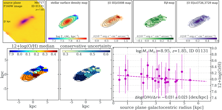
Figure A1. Source-plane metallicity radial gradient measurement of one highly anisotropically magnified galaxy (MACS 0717–ID 01131) in our sample. Its image-plane metallicity radial gradient measurement is presented in Figure B1. Top, from left to right: the source-plane reconstructed 2D maps of  -band surface brightness, stellar surface density (
 ), and surface brightness of emission lines
 ![$[{\rm{O}}\,{\rm\small{III}}]$](https://content.cld.iop.org/journals/0004-637X/900/2/183/revision1/apjabacceieqn847.gif) , Hβ, and
, Hβ, and ![$[{\rm{O}}\,{\rm\small{II}}]$](https://content.cld.iop.org/journals/0004-637X/900/2/183/revision1/apjabacceieqn848.gif) . These 2D maps are arranged on the same spatial scale with a scale bar of 1 kpc shown in the leftmost panel. The black contours mark the deprojected galactocentric radii with 1 kpc intervals, with galaxy inclination taken into account. Note that the black radius contours in Figure B1 are obtained from relensing the contours shown in this figure to the image plane of this galaxy. Bottom: metallicity map and radial gradient determination for this galaxy in its source plane. We again use Voronoi tessellation to divide its source-plane reconstructed spatial extent into bins with a constant S/N of 5 on
. These 2D maps are arranged on the same spatial scale with a scale bar of 1 kpc shown in the leftmost panel. The black contours mark the deprojected galactocentric radii with 1 kpc intervals, with galaxy inclination taken into account. Note that the black radius contours in Figure B1 are obtained from relensing the contours shown in this figure to the image plane of this galaxy. Bottom: metallicity map and radial gradient determination for this galaxy in its source plane. We again use Voronoi tessellation to divide its source-plane reconstructed spatial extent into bins with a constant S/N of 5 on ![$[{\rm{O}}\,{\rm\small{III}}]$](https://content.cld.iop.org/journals/0004-637X/900/2/183/revision1/apjabacceieqn849.gif) , the same as used in the gradient measurement in the image plane. In the right panel, the metallicity measurements in these source-plane Voronoi bins are plotted as magenta points. The dashed magenta line denotes the linear regression, with the corresponding slope shown at the bottom. The metallicity gradient measured in the source plane is
, the same as used in the gradient measurement in the image plane. In the right panel, the metallicity measurements in these source-plane Voronoi bins are plotted as magenta points. The dashed magenta line denotes the linear regression, with the corresponding slope shown at the bottom. The metallicity gradient measured in the source plane is ![${\rm{\Delta }}\mathrm{log}({\rm{O}}/{\rm{H}})/{\rm{\Delta }}r=-0.031\pm 0.023\,[\mathrm{dex}\,{\mathrm{kpc}}^{-1}]$](https://content.cld.iop.org/journals/0004-637X/900/2/183/revision1/apjabacceieqn850.gif) , in agreement with the gradient measured in the image plane, i.e., Δ log(O/H) / Δr = −0.055 ± 0.028 [dex kpc−1].
, in agreement with the gradient measured in the image plane, i.e., Δ log(O/H) / Δr = −0.055 ± 0.028 [dex kpc−1].
Download figure:
Standard image High-resolution imageFor the galactocentric distance scale of each individual source-plane Voronoi bin, we again rely on the 2D elliptical Gaussian function fit to the source-plane stellar mass surface density map of this galaxy21 (see the second panel in Figure A1). This fitting procedure yields the best-fit inclination, axis ratio, and major-axis orientation of the galaxy so that we not only take out the effect of lensing distortion but also take into account the projection effect when determining the source intrinsic morphology. At last, the radial gradient can be given by a linear regression to the metallicity estimates in all source-plane Voronoi bins.
For our exemplary differentially magnified source MACS 0717–ID 01131, the metallicity gradient measured in its source plane is ![${\rm{\Delta }}\mathrm{log}({\rm{O}}/{\rm{H}})/{\rm{\Delta }}r=-0.031\pm 0.023\,[\mathrm{dex}\,{\mathrm{kpc}}^{-1}]$](https://content.cld.iop.org/journals/0004-637X/900/2/183/revision1/apjabacceieqn852.gif) , in agreement at a 1σ confidence level with the gradient measured in the image plane, i.e.,
, in agreement at a 1σ confidence level with the gradient measured in the image plane, i.e., ![${\rm{\Delta }}\mathrm{log}({\rm{O}}/{\rm{H}})/{\rm{\Delta }}r=-0.055\,\pm 0.028[\mathrm{dex}\,{\mathrm{kpc}}^{-1}]$](https://content.cld.iop.org/journals/0004-637X/900/2/183/revision1/apjabacceieqn853.gif) (shown in Figure B1 and given in Table A1). We verified that this difference (≲0.03
(shown in Figure B1 and given in Table A1). We verified that this difference (≲0.03  , compatible within 1σ) is typical for the few highly anisotropically magnified galaxies in our sample. In fact, the metallicity radial gradient measurement in this galaxy was presented in our previous work (Jones et al. 2015). Using half of the grism data (two orbits of G141 and five orbits of G102) available at that time, Jones et al. (2015) estimated the radial metallicity gradient of this galaxy to be
  from metallicities measured in individual spatial pixels and
  from metallicities derived in radial annuli. We see that our updated results derived in both the image and source planes presented in this work are compatible with previous measurements within the measurement uncertainties.
Appendix B: A Summary of the Data Products and Analysis Results for the Full Metallicity Gradient Sample Presented in This Paper (Online Material)
In Figure B1 and its online figure set, we present the source 1D/2D grism spectra, color-composite image, stellar surface density stamp, and emission line maps, as well as the metallicity map and radial metallicity gradient measurements for the entire sample. Following the conventions adopted in Figures 2 and 7, we first show the 1D and 2D G102–G141 spectra at two separate PAs. Note that due to grism defects and/or falling outside the WFC3 FoV, some sources (i.e., A2744–ID 00144, A2744–ID 01897, and RX J1347–ID 00664) only have coverage from one of the orients. Beneath the spectra, we show the source 2D stamps. For sources at z ≲ 1.6, we display their Hα map, whereas for sources at higher redshifts, the Hγ map is shown instead, since Hα has already redshifted out of the wavelength coverage of HST grisms. The bottom panels show the metallicity map and radial gradient measurements.

Figure B1.
The source ID 01131 in the field of MACS 0717.5+3745 is shown. (The complete figure set (65 images) is available.)
Download figure:
Standard image High-resolution imageFootnotes
- 12
Throughout this paper, we use metallicity to stand for gas-phase oxygen abundance unless otherwise specified.
- 13
- 14
- 15
Specifically, step (1) includes bad-pixel/persistence masking, bias correction, dark subtraction, cosmic-ray flagging, relative/absolute astrometric alignment, flat-fielding, master/variable sky background subtraction, geometric distortion correction, extraction of source catalogs, and segmentation images at visit levels.
- 16
Out of the 37 sources in this redshift range, 31 have Hα detected with S/N ≳ 10.
- 17
We note that in the most up-to-date version of Grizli, the subtraction of
![$[{\rm{O}}\,{\rm\small{III}}]$](data:image/png;base64,iVBORw0KGgoAAAANSUhEUgAAAAEAAAABCAQAAAC1HAwCAAAAC0lEQVR42mNkYAAAAAYAAjCB0C8AAAAASUVORK5CYII=) λ4960 is implemented. However Grizli's automatic subtraction is based on a spatial model of λ4960 emission, which is different from our procedure presented here.
λ4960 is implemented. However Grizli's automatic subtraction is based on a spatial model of λ4960 emission, which is different from our procedure presented here. - 18
- 19
Only 3/11 gradients reported in Leethochawalit et al. (2016) have
measured. - 20
Here we use the SED-derived SFR, i.e., SFRS, in Table A1 for our galaxies to be self-consistent throughout the combined sample.
- 21
Note that this fitting is always performed for metallicity gradient measurements in the image plane, such that the black contours shown in all image-plane 2D maps for our sample galaxies are obtained by relensing the corresponding best-fit source-plane deprojected galactocentric radius contours.
![$[{\rm{O}}\,{\rm\small{III}}]$](https://content.cld.iop.org/journals/0004-637X/900/2/183/revision1/apjabacceieqn50.gif)
![$[{\rm{O}}\,{\rm\small{III}}]$](https://content.cld.iop.org/journals/0004-637X/900/2/183/revision1/apjabacceieqn51.gif)
![$[{\rm{N}}\,{\rm\small{II}}]$](https://content.cld.iop.org/journals/0004-637X/900/2/183/revision1/apjabacceieqn138.gif)
