


Abstract
We report the discovery and analysis of the planetary microlensing event OGLE-2017-BLG-0406, which was observed both from the ground and by the Spitzer satellite in a solar orbit. At high magnification, the anomaly in the light curve was densely observed by ground-based-survey and follow-up groups, and it was found to be explained by a planetary lens with a planet/host mass ratio of  from the light-curve modeling. The ground-only and Spitzer-"only" data each provide very strong one-dimensional (1D) constraints on the 2D microlens parallax vector
  . When combined, these yield a precise measurement of
  and of the masses of the host
  and planet Mplanet = 0.41 ± 0.05 MJup. The system lies at a distance DL = 5.2 ± 0.5 kpc from the Sun toward the Galactic bulge, and the host is more likely to be a disk population star according to the kinematics of the lens. The projected separation of the planet from the host is
  (i.e., just over twice the snow line). The Galactic-disk kinematics are established in part from a precise measurement of the source proper motion based on OGLE-IV data. By contrast, the Gaia proper-motion measurement of the source suffers from a catastrophic 10σ error.
Export citation and abstract BibTeX RIS
1. Introduction
Gravitational microlensing has a unique strength in its sensitivity to planets with masses as low as Earth mass (Bennett & Rhie 1996) just beyond the snow line (Gould & Loeb 1992), where the core accretion theory of planetary formation predicts the most efficient planet formation (Ida & Lin 2005). Because it does not rely on the light from the host star, microlensing can detect the planets orbiting around faint stars like M-dwarfs and brown dwarfs, and can even detect free-floating planets (Sumi et al. 2011; Mróz et al. 2017, 2018, 2019, 2020). Microlensing can also detect planets in the Galactic bulge because microlensing events can be caused by stars at any distance between Earth and the Galactic bulge, where most of the stars that act as sources lie. This is complementary to other planet detection techniques, such as the radial velocity (Butler et al. 2006) and transit (Borucki et al. 2011) methods, which are most sensitive to planets in short period orbits. Therefore, the microlensing method is essential for the complete demographic census of Galactic planetary systems (Gaudi 2012; Tsapras 2018).
Several statistical studies based on the discovered microlensing planets have been conducted and revealed the planet occurrence rates beyond the snow line (Gould et al. 2010; Sumi et al. 2010; Cassan et al. 2012; Shvartzvald et al. 2016) and the possible paucity of planets in the Galactic bulge (Penny et al. 2016). One of the most important microlensing statistical results is that of Suzuki et al. (2016), who found a clear break and likely peak in the planet-host mass ratio function at a mass ratio of q ∼ 10−4 using 30 exoplanets detected by microlensing. This peak was confirmed by Udalski et al. (2018) and Jung et al. (2018), who determined that the peak occured at a mass ratio of q ≈ 6 × 10⁻⁵. A comparison of the Suzuki et al. (2016) results to population synthesis models based on the core accretion theory (Suzuki et al. 2018) reveals a discrepancy between the smooth mass ratio distribution for the microlens planets and the predicted deficit of planets, with mass ratios lying in the range of  . This predicted gap in the mass ratio distribution (Ida & Lin 2004) is due to the runaway gas accretion process (Pollack et al. 1996; Lissauer et al. 2009), which has long been considered a fundamental aspect of the core accretion theory. So, the microlensing results seem to imply that a major change in the theory is needed. In fact, recent three-dimensional high-resolution numerical calculations (Szulágyi et al. 2014; J. Szulágyi et al. 2020, in preparation) indicate that runaway gas accretion often halted or decreased due to the circumplanetary disk formation and suggest that earlier, lower resolution three-dimensional calculations had numerical artifacts that favored the runaway gas accretion scenario. Comparison of the population synthesis results to ALMA protoplanetary disk observations also support this conclusion (Nayakshin et al. 2019).
Microlensing light-curve models provide the lens planet-host mass ratios, but they do not usually provide the lens mass and distance. To measure the properties of lens systems, one needs additional observables that yields mass–distance relation of the lens systems, such as the angular Einstein ring radius θE and the microlens parallax πE. The measurement of the θE or πE values yields the following mass–distance relations,

where DL is the lens distance and the source distance, DS, is known (approximately). If the apparent K-band magnitude of the lens star  is measured, then we have a mass–distance relation given by
  , where
  is a K-band mass–luminosity relation and
  is a model of the extinction in the foreground of the lens star. Measurements of the lens brightness in other passbands yield independent mass–distance relations. Combining any two of these mass–distance relations will yield the lens mass ML and distance DL. The most elegant solution is obtained if both the angular Einstein radius, θE, and the microlensing parallax, πE, are measured because this distance dependence cancels, enabling unique determinations of ML and DL by the following relations,

where  and πS = 1 au/DS (Gould 1992, 2000). For binary events, θE can be routinely measured by the source radius crossing time, t*, provided that the source crosses a caustic curve or closely approaches to a caustic cusp. This gives θE = θ* tE/t*, where
  is the angular radius of the source, which can be determined from the light-curve model values for the source brightness and color (Albrow et al. 1998; Yoo et al. 2004).
It can be challenging to obtain the measurements necessary for the other mass–distance relations, aside from the θE relation. Detecting the host star is nearly impossible for bright source stars, and a unique identification of the host star can be difficult if the source star is bright (i.e., a giant star) or if the relative lens-source proper motion is not big enough to resolve the lens and source (Bhattacharya et al. 2017; Koshimoto et al. 2017, 2020). Because the lens-source separation increases as time passes after an event, there are an increasing number of planetary events with mass measurements from host star brightness measurements (Bennett et al. 2006, 2015, 2020; Batista et al. 2015; Bhattacharya et al. 2018; Vandorou et al. 2019), and this is the method that is expected to make most of the exoplanet mass measurements for WFIRST (Bennett & Rhie 2002; Bennett et al. 2007; Spergel et al. 2015).
The microlensing parallax effect has traditionally been measured due to the effects of the orbital motion of Earth. Dong et al. (2009) made the first such measurement on OGLE-2005-BLG-071 (only the second planet detected by microlensing; Udalski et al. 2005), which was made possible in part by the exceptionally large parallax.61 However, in general, this annual parallax effect can only be measured for a subset of planetary microlensing events: events that have long durations, like OGLE-2006-BLG-109 (Gaudi et al. 2008; Bennett et al. 2010) and OGLE-2007-BLG-349 (Bennett et al. 2016), have bright source stars and moderately long durations, like MOA-2009-BLG-266 (Muraki et al. 2011) and OGLE-2012-BLG-0265 (Skowron et al. 2015), or have very special lens-source geometries, such as MOA-2013-BLG-605 (Sumi et al. 2016) and OGLE-2013-BLG-0341 (Gould et al. 2014).
However, πE can also be measured by simultaneously observing lensing events from two well-separated (∼au) observatories (Refsdal 1966). Since 2014, almost 1000 events, including both single and binary events, were simultaneously observed from the ground and the Spitzer Space Telescope (Yee et al. 2015a; Zhu et al. 2017). Spitzer observations helped determine the distance to the lens for more than a hundred of those events. To date, ten planetary events were observed by Spitzer. Seven of these are located in the Galactic disk: OGLE-2014-BLG-0124 (Udalski et al. 2015b; Beaulieu et al. 2018), OGLE-2015-BLG-0966 (Street et al. 2016), OGLE-2017-BLG-1140 (Calchi Novati et al. 2018), OGLE-2016-BLG-1067 (Calchi Novati et al. 2019), OGLE-2016-BLG-1195 (Bond et al. 2017; Shvartzvald et al. 2017), KMT-2018-BLG-0029 (Gould et al. 2020), and Kojima-1 (Nucita et al. 2018; Fukui et al. 2019; Zang et al. 2020). The lens systems for events OGLE-2016-BLG-1190 (Ryu et al. 2017), OGLE-2018-BLG-0596 (Jung et al. 2019), and OGLE-2018-BLG-0799 (W. Zang et al. 2020, in preparation) are reported to be in the Galactic bulge. While observations from Spitzer make it easier to measure the small πE values for bulge lens systems, this ability is undermined by the requirement that events should be discovered at least ∼1 week before Spitzer observations can be requested (Figure 1 from Udalski et al. 2015b). This, combined with the limited 40 day Spitzer observing window for bulge events, leads to incomplete light curves, which can make parallax measurements difficult.
In this paper, we report the discovery and analysis of the planetary microlensing event OGLE-2017-BLG-0406, which was observed both from the ground and in space using the Spitzer telescope. The anomaly in the light curve was well covered by ground-based observations. The additional Spitzer data constrained the parallax parameters—hence the mass and the distance of the lens systems. We describe the ground-based and space-based observations in Section 2 and the data reductions in Section 3. In Section 4, we describe our light-curve modeling conducted for the ground-based data. We present our Spitzer parallax analysis in Section 5. In Sections 6 to 8, we present the determinations of source properties and lens properties. Finally, we discuss and summarize the results in Section 9.
2. Observations
2.1. Ground-based Observation
The microlensing event OGLE-2017-BLG-0406 was first discovered on March 27 (HJD' = HJD-2,450,000 = 7839) by the Optical Gravitational Lensing Experiment (OGLE) collaboration at (R.A., decl.)(J2000)=( ,
,  ) or (l, b) = (0
 3601, − 24164) in Galactic coordinates, as alerted by the OGLE Early Warning System (Udalski 2003). The event lies in the OGLE-IV field BLG506, and the observations were conducted at the cadence of once per hour by using the 1.3 m Warsaw telescope located at Las Campanas Observatory in Chile, equipped with a 1.4 deg2 field-of-view CCD camera. The Microlensing Observations in Astrophysics (MOA) group independently discovered this event on May 5 (HJD' = 7879) by using the MOA alert system (Bond et al. 2001) and identified it as MOA-2017-BLG-233. MOA observed this event with 15 minutes cadence by using MOA-II telescope at Mt. John University Observatory in New Zealand, equipped with 2.2 deg2 field-of-view camera MOA-camIII (Sako et al. 2008). Most observations were conducted in the customized MOA-Red wide band, which is the sum of the standard Cousins R and I bands with occasional observations in the Johnson V band. The event was also independently discovered as KMT-2017-BLG-0243 by the Korean Microlensing Network (KMTNet: Kim et al. 2016) survey using its post-season event finder (Kim et al. 2018). KMTNet observes toward the Galactic bulge by using three 1.6 m telescopes equipped with 4 deg2 camera at the Cerro Tololo Inter-American Observatory in Chile (CTIO: KMT-C), the South African Astronomical Observatory in South Africa (SAAO: KMT-S), and the Siding Spring Observatory in Australia (SSO: KMT-A). Because this event was in an overlapping region between two fields (KMTNet BLG02 and BLG42), the observations were conducted at a 15 minute cadence.
On June 2 (HJD' = 7907), the Microlensing Follow-up Network (μFUN) collaboration issued an alert that the event was peaking at a high magnification, which means that there is a high probability that the light curve will show an anomaly if the lens star hosts a planet (Griest & Safizadeh 1998). After the alert, μFUN, the Microlensing Network for the Detection of Small Terrestrial Exoplanet (MiNDSTEp) collaboration and Las Cumbres Observatory (LCO) global network of telescope collaboration started high-cadence follow-up observations. μFUN used the following telescopes: the 1.3 m CTIO telescope in Chile, the 0.41 m Auckland telescope and the 0.36 m Farm Cove telescope in New Zealand, and the 0.30 m Perth Exoplanet Survey Telescope (PEST), and the 0.25 m Craigie telescope in Australia. MiNDSTEp used the 1.54 m Danish Telescope at La Silla Observatory in Chile. LCO used the 1.0 m telescopes at CTIO in Chile and at SSO in Australia. Figure 1 shows the light curve of the event.
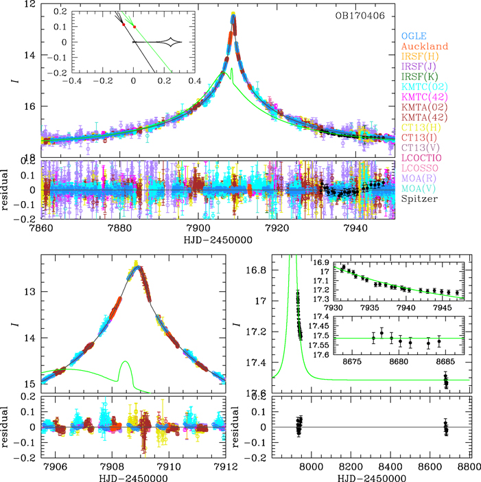
Figure 1. Observed light curve of OGLE-2017-BLG-0406 and best-fit model light curve for the Wide (+,+) model. Data points from different collaborations are shown with different colors. The blue and green solid lines are the model light curves for the ground and Spitzer observations. The bottom left and right panels show a close-up of the anomaly and Spitzer observations with the residuals from the best-fit model, respectively. The insert on the top panel shows the caustic structure.(The data used to create this figure are available.)
Download figure:
Standard image High-resolution imageOn June 4 (HJD' = 7909), deviations from a single-lens fit were noticed just after the peak by the MOA observer. Then the first planetary model was circulated by V. Bozza, and it was confirmed by several modelers. Because the event was very bright (∼12.5 mag in I band), some images taken with normal exposure time by survey telescopes were saturated.
We also obtained three near-infrared images taken at different epochs (HJD' ∼ 7911, 7918 and 7942). The observations were made with SIRIUS, a simultaneous imager in J, H, and KS bands, covering an area 7.7 × 7.7 arcmin2 with a pixel scale of 0 45 (Nagayama et al. 2003) on the 1.4 m InfraRed Survey Facility (IRSF) telescope at SAAO. The observations were conducted to measure the source color rather than for light-curve modeling. The data sets are listed in Table 1.
Table 1. The Data Sets Used to Model the OGLE-2017-BLG-0406 Light Curve and the Error Correction Parameters
| Telescope | Filter |

|
k |

|
|---|---|---|---|---|
| OGLE | I | 6185/6185 | 1.441 | 0.003257 |
| MOA | Red | 14611/14611 | 1.970 | 0.003257 |
| V | 315/315 | 1.794 | 0.003257 | |
| KMT-C02 | I | 1558/1558 | 2.537 | 0.003257 |
| KMT-C42 | I | 1713/1713 | 1.897 | 0.003257 |
| KMT-A02 | I | 1903/1903 | 2.590 | 0.003257 |
| KMT-A42 | I | 2068/2068 | 2.550 | 0.003257 |
| KMT-S02 | I | 0/2485 | ||
| KMT-S42 | I | 0/2481 | ||
| Danish | I | 0/200 | ||
| LCO-CTIO | I | 296/296 | 1.323 | 0.003257 |
| LCO-SSO | I | 464/464 | 1.644 | 0.003257 |
| Auckland | R | 82/82 | 2.280 | 0.003257 |
| Craigie | clear | 0/677 | ||
| Farm Cove | clear | 0/31 | ||
| PEST | clear | 0/262 | ||
| CTIO | I | 21/21 | 0.860 | 0.003257 |
| V | 7/7 | 0.760 | 0.003257 | |
| H | 92/93 | 1.700 | 0.003257 | |
| IRSF | J | 3/3 | 1.000 | 0.000 |
| H | 3/3 | 1.000 | 0.000 | |
| KS | 3/3 | 1.000 | 0.000 | |
| Spitzer | L | 21/21 | 3.120 | 0.003257 |
Download table as: ASCIITypeset image
2.2. Space-based Observation
OGLE-2017-BLG-0406 was observed by the Spitzer space telescope with the 3.6 μm (L-band) channel of the IRAC camera. Spitzer started to observe this event on June 26 (HJD' = 7931), which was about 3 weeks after the peak because this was the first date that the target was visible in the Spitzer image. This event was chosen for Spitzer observations as part of a long-term (2014–2019) program, according to the protocols of Yee et al. (2015a). Specifically, it met objective criteria defined by Yee et al. (2015a), which meant that it had to be chosen for observations and observed at a specified cadence, independent of whether it had a planet or not. Accordingly, it was observed approximately once per day for the first 4 weeks, but not the final 2 weeks of the program in 2017.
In 2019 (i.e., the final Spitzer microlensing season), essentially all planetary events from 2014 to 2018 were observed for about a week at baseline, primarily to check for systematics in the light curves, in part because of concerns raised by Koshimoto & Bennett (2019). See Gould et al. (2020) for further discussion. OGLE-2017-BLG-0406 was observed seven times under this program, meaning that there are a total of 28 data points. As discussed in Section 9.1, these seven points must be excluded when determining whether OGLE-2017-BLG-0406Lb can enter the Spitzer-statistical sample. For the role of these data in the analysis of systematic effects, see the Appendix.
3. Data Reduction
The great majority of the ground-based data were reduced using the pipelines developed by the individual collaborations based on difference image analysis (DIA) method developed by Tomaney & Crotts (1996) and Alard & Lupton (1998). The OGLE I-band data were reduced by the OGLE DIA (Woźniak 2000) photometry pipeline (Udalski et al. 2015a). The MOA-Red and V-band data were reduced by the MOA DIA pipeline (Bond et al. 2001). KMTNet-I-band data were reduced with their pySIS photometry pipeline (Albrow et al. 2009). μFUN data were reduced using DoPhot (Schechter et al. 1993), and LCO data were reduced using pySIS (Albrow et al. 2009). Danish data were reduced using an updated version of DanDIA (Bramich 2008). IRSF images were reduced using the standard IRSF pipeline and MOA DIA pipeline. Spitzer L-band data was reduced using methods described in Calchi Novati et al. (2015).
The error bars must be renormalized to accurately estimate the uncertainties. We use the following formula to rescale the errors,  , where σi and
  are original and renormalized error bars in magnitudes, and k and emin are rescaling factors (Bennett et al. 2008). The value of emin represents systematic errors that dominate at high magnification or when the target is very bright. First, we fit all the light curves to find a tentative best-fit model. Then we apply emin = 0.003257 and choose k values to give χ2/dof = 1 for a preliminary best-fit model. Finally, all the normalized light curves are fit again and we get the final best-model. In this process, we find that there are systematics in the data from Danish, Craigie, Farm Cove, and PEST. Also, Danish data are not consistent with the OGLE and LCO-CTIO data. Hence, they are not used for the analysis. We note that the data from KMT-S are not used because of the systematics that mimic the parallax signal, as described in Section 4. The data sets we used, together with the values of k and
  , are shown in Table 1. We also note that for the OGLE-IV data, we check the standard error correction procedure described in Skowron et al. (2016a) and find that the resulting error bars are similar to those estimated in this work. We choose k = 1 and emin = 0 for IRSF data.
4. Ground-based Light-curve Analysis
For the point-source point-lens model, one needs three parameters to characterize the microlens light curve: t0, the time of closest approach of the source to the lens mass; u0, the impact parameter in units of the angular Einstein radius θE; and tE, the Einstein radius crossing time. For the binary-lens model, one needs three additional parameters: q, the planet/host mass ratio; s, the projected planet—star separation in units of the Einstein radius; and α, the angle of the source trajectory relative to the binary-lens axis. When we take account of the finite-source effect and the parallax effect, the angular radius of the source star in units of θE, ρ, and the north and east components of the microlensing parallax vector,  and
and  , are added for each case. The model light curve is given by

where F(t) is the flux at time t, A(t) is the magnification of the source star at t, and  and
and  are the baseline fluxes from the source and blend stars for each data set, i, respectively.
We use linear limb-darkening models for the source star. The effective temperature of the source star estimated from the extinction-corrected source color,  , as described in Section 6, is
  (González Hernández & Bonifacio et al. 2009). Rounding to the nearest Teff given in Claret (2000) and assuming surface gravity
 ![$\mathrm{log}[g/(\mathrm{cm}\ {{\rm{s}}}^{-2})]=4.5$](https://content.cld.iop.org/journals/1538-3881/160/2/74/revision1/ajab9ac3ieqn26.gif) , and metallicity
, and metallicity ![$\mathrm{log}[{\rm{M}}/{\rm{H}}]=0$](https://content.cld.iop.org/journals/1538-3881/160/2/74/revision1/ajab9ac3ieqn27.gif) , we selected limb-darkening coefficients uλ to be uI = 0.6049, uRed = 0.6534, uV = 0.7796, uR = 0.7081, uJ = 0.4896, uH = 0.4252, and
, we selected limb-darkening coefficients uλ to be uI = 0.6049, uRed = 0.6534, uV = 0.7796, uR = 0.7081, uJ = 0.4896, uH = 0.4252, and  , respectively (Claret 2000). The MOA-Red value is the mean of the R- and I-band values.
We first conduct the light-curve modeling by only using ground-based data. Our light-curve modeling was done using the image-centered ray-shooting method (Bennett & Rhie 1996; Bennett 2010) and the Markov Chain Monte Carlo (MCMC) algorithm (Verde et al. 2003). Note that the source and blend flux parameters are not MCMC parameters, but are fit linearly to each model following Rhie et al. (1999). To find the global best-fit model, we first conduct a grid search by fixing three parameters (q, s, α) while the other parameters (t0, tE, u0, ρ) are allowed to be free. Next, we search for the best-fit model by refining all parameters for those models with the 100 smallest χ2 values as initial parameters. From this modeling, we find a planetary model that has the best-fit values of q ∼ 0.0007 and s ∼ 1.128. The best-fit parameters are shown in Table 2. Because the source crosses the central caustic very close to the lens host star as seen in Figure 1, the finite-source effect is well measured. The Δχ2 between the best-fit model and the single-lens model is more than 20,000. Thus, the planetary signal is detected confidently. We also explore the binary-source single-lens model (Gaudi 1998) and find that the model is ruled out by Δχ2 > 3000.
Table 2. Standard Models
| Parameters | Wide ( ) ) |
Close ( ) ) |
|---|---|---|

|
29272.22/29285 | 29325.836/29285 |
t0 
|
7908.809 ± 0.001 | 7908.810 ± 0.001 |
u0 
|
9.437 ± 0.028 | 9.454 ± 0.029 |
 
|
37.043 ± 0.082 | 36.994 ± 0.083 |
| s | 1.129 ± 0.001 | 0.895 ± 0.001 |
q 
|
7.024 ± 0.090 | 6.876 ± 0.091 |
α 
|
0.993 ± 0.001 | 0.993 ± 0.002 |
ρ 
|
5.861 ± 0.025 | 5.830 ± 0.025 |

|
1.462 ± 0.004 | 1.464 ± 0.004 |

|
0.102 ± 0.004 | 0.100 ± 0.004 |
 
|
0.217 ± 0.001 | 0.216 ± 0.001 |
Note.  is a derived quantity and is not fitted independently. All fluxes are on an 18th mag scale (e.g.,
  ).
).
Download table as: ASCIITypeset image
High-magnification planetary microlensing events often have a so-called close-wide degeneracy because the structures near the central caustic are very similar to each other for  , particularly for s ≪ 1 and s ≫ 1 (Griest & Safizadeh 1998; Dominik 1999; Chung et al. 2005). We search for the model with s < 1 and find the model that has the best-fit values of q ∼ 0.0007 and s ∼ 0.895. But this close model has worse χ2 compared to the best-fit wide model by Δχ2 ∼ 41. This difference mostly comes from the data near the peak. Thus, we exclude the close model because of its poor fit.
When  is large, we have a chance to measure the orbital parallax effect, which is caused by the acceleration of Earth's orbital motion (Gould 1992; Alcock et al. 1995). We do not expect a significant orbital microlensing parallax signal for such a short event, in the middle of the season, because the acceleration of Earth projected to the bulge is the smallest. We begin by doing a parallax fit without the Spitzer data to independently assess parallax constraints coming from the ground-based data. We conduct the parallax fit by adding the two additional parameters,
  and
and  . In the first iteration, we found a model with a large πE value of ∼0.4. However, the Δχ2 between the standard model and the parallax model comes mostly from KMT-S data, and it was not consistent with the other data sets. Also, the differences were from the baseline. Hence, we conduct parallax analysis without the KMT-S data set because we think that there is a systematic error in the data set, which mimics the deviation caused by the parallax effect. Then we tried the parallax fit again and obtained a smaller πE value of ∼0.2. The best-fit parameters are shown in Table 3. While the improvement in
  is relatively small (
 ), Figures 2 and 3 show that there is a strong one-dimensional (1D) parallax constraint, which arises from the asymmetry in the light curve induced by the instantaneous acceleration of Earth around the peak of the event (Gould et al. 1994). The relatively small Δχ2 simply reflects the fact that this 1D constraint happened to pass close to the origin. We will return to the role of this 1D parallax constraint after including Spitzer data into the analysis.

Figure 2. OGLE-2017-BLG-0406 parallax contours for the W+ solution. Left: the ground-only (elliptical) contours are derived from the covariance matrix from the MCMC, while the Spitzer-"only" (arc-like) contours are derived from the analytical expression in Equation (7). The colors (black, red, yellow, green, cyan, blue, magenta) represent  . Note that the 1σ contours for the ground-only and Spitzer-"only" measurements overlap. Right: Colored contours are the
  values for the sum of the two
  distributions that are shown to the left. Despite the fact the each set of contours on the left provides essentially 1D information, the combination is well constrained in both dimensions. The white ellipses represent the 1σ, 2σ, and 3σ contours from the combined numerical fit to all of the data. The semi-analytic approach (colored contours) provides a very good, although not perfect, representation of the full numerical result. This shows that the semi-analytic approach enables one to accurately trace the information flow.
Download figure:
Standard image High-resolution image
Figure 3. OGLE-2017-BLG-0406 parallax contours for the W− solution. Similar to Figure 2.
Download figure:
Standard image High-resolution imageTable 3. Parallax Models for Ground-only Data
| Parameters | Wide 
|
Wide 
|
Close 
|
Close 
|
|---|---|---|---|---|

|
29272.225/29283 | 29273.381/29283 | 29318.530/29283 | 29318.828/29283 |
t0 
|
7908.809 ± 0.001 | 7908.809 ± 0.001 | 7908.809 ± 0.001 | 7908.809 ± 0.001 |
u0 
|
9.402 ± 0.032 | −9.447 ± 0.030 | 9.432 ± 0.027 | −9.419 ± 0.030 |
 
|
37.168 ± 0.096 | 37.042 ± 0.091 | 37.075 ± 0.076 | 37.119 ± 0.091 |
| s | 1.129 ± 0.001 | 1.130 ± 0.001 | 0.895 ± 0.001 | 0.895 ± 0.001 |
q 
|
6.972 ± 0.093 | 7.073 ± 0.092 | 6.894 ± 0.089 | 6.831 ± 0.090 |
α 
|
0.991 ± 0.001 | −0.992 ± 0.002 | 0.993 ± 0.002 | −0.992 ± 0.002 |
ρ 
|
5.832 ± 0.025 | 5.874 ± 0.025 | 5.822 ± 0.025 | 5.809 ± 0.025 |

|
0.179(0.167) ± 0.094 | 0.157(0.168) ± 0.066 | 0.137(0.121) ± 0.031 | 0.198(0.168) ± 0.065 |

|
0.097(0.089) ± 0.037 | 0.097(0.088) ± 0.026 | 0.064(0.070) ± 0.014 | 0.098(0.086) ± 0.027 |

|
0.204(0.193) ± 0.093 | 0.185(0.191) ± 0.069 | 0.151(0.141) ± 0.030 | 0.221(0.189) ± 0.068 |

|
0.494(0.554) ± 0.481 | 0.554(0.507) ± 0.123 | 0.438(0.538) ± 0.124 | 0.459(0.498) ± 0.155 |

|
1.457 ± 0.004 | 1.463 ± 0.004 | 1.460 ± 0.004 | 1.459 ± 0.004 |

|
0.107 ± 0.004 | 0.101 ± 0.004 | 0.104 ± 0.003 | 0.105 ± 0.004 |
 
|
0.217 ± 0.001 | 0.218 ± 0.001 | 0.216 ± 0.001 | 0.216 ± 0.001 |
Note. Mean values from the MCMC are shown in parentheses. All other values are from the best-fit model.  ,
,  , and
, and  are derived quantities and are not fitted independently. All fluxes are on an 18th mag scale (e.g.,
  ).
).
Download table as: ASCIITypeset image
5. Spitzer Parallax Analysis
5.1. Spitzer-"only" Parallax
In principle, we could now proceed to incorporate the Spitzer data into a joint fit together with the ground-based data. We will do so in Section 5.2. First, however, it is important to examine how the Spitzer data and the ground-based data contribute information to the parallax measurement. The principal reason for doing so is that both data sets can be subject to systematic errors, which are of very different types and can affect the parallax measurement very differently. An important check for such systematics is whether the parallax information derived from each data set is consistent with the other. Failure of this test would provide clear evidence for systematics in one or both data sets. In addition, we will ultimately be making somewhat separate use of the magnitude and direction of the parallax vector. In order to understand how secure each of these components is, we will need to trace their origins in different combinations of Spitzer-based and ground-based information.
In Section 4, we showed that the ground-based data yielded essentially one-dimensional parallax information, with  (the component parallel to the instantaneous projected direction of the Sun at t0) measured about nine (for W+) or five (for W-) times more precisely than the orthogonal component
  . This is because the information for the latter comes from further out in the wings of the light curve (Smith et al. 2003; Gould 2004), which, for events like OGLE-2017-BLG-0406 that are not extremely long, is generally quite faint. This also means that the
  component is much more sensitive to long-term trends in the data. In the present case, for which
  , this means that the direction of the ground-based parallax vector is determined much more confidently than its magnitude.
The Spitzer light curves can also be affected by long-term trends in the data, which can affect the parallax measurement. In their analysis of 50 Spitzer events from 2015, Zhu et al. (2017) identified five with obvious trends in the data, and Koshimoto & Bennett (2019) identified 14 more. There is only one case for which the causes of such trends have been investigated: KMT-2018-BLG-0029 (Gould et al. 2020). In that case, bright nearby blends with poorly determined positions were found to be likely to have generated trends, as the Spitzer camera rotated during the season. Because the source was faint and not well magnified, the trends were about 30% of the total observed flux variations. Nevertheless, after the trends were removed, the amplitude of the parallax measurement only changed by 20% (about 2σ). Thus, it is important to both carefully evaluate and minimize the impact of potential Spitzer systematics.
Refsdal (1966) originally analyzed satellite parallaxes prior to the time (Gould 1992) that it was recognized that the ground-based light curve alone would have any parallax information. Hence, although not explicitly stated, his was in essence a satellite-"only" analysis. The ground-based parameters  were directly compared to the satellite parameters
  to produce the parallax measurement

where D⊥is the projected separation of the satellite from Earth and where it was implicitly assumed that the Einstein timescales were the same  . The implicit idea (as illustrated in Figure 1 of Gould 1994 and first realized in Figure 1 of Yee et al. 2015b) is that
  would be "observables" from the satellite, just as the corresponding quantities were from Earth. Note that Equation (4) has a fourfold degeneracy because u0 is a signed quantity but only
  is determined directly from the light curve. See Figure 4 of Gould (2004) for the sign convention.
However, in real Spitzer microlensing events, the peak is very often not observed from space, primarily because there is a ∼3–10 day time delay between identifying the event and initiating satellite observations (Figure 1 from Udalski et al. 2015b). Hence, while Equation (4) remains formally valid, it may no longer express the parallax measurement in terms of "observables," because (t0, u0)sat may not be separately determined.
Gould (2019) generalized Refsdal's satellite-"only" analysis to the case of satellite data streams that did not cover the peak. He showed that if the source flux in the satellite observations was known and the baseline flux was measured, then each satellite measurement at finite magnification yields an exactly circular degeneracy in the  plane. In the presence of measurement errors, these circles become finite annuli. If these measurements cover the peak, then the corresponding circles intersect in exactly two places, which then reproduces the Refsdal (1966) fourfold degeneracy (two pairs, one each for
  ). See Figure 3 of Gould (2019). On the other hand, the osculating circles from a series of late-time measurements combine to form an extended arc. See Figure 1 of Gould (2019). Such arcs may yield exquisite 1D constraints on
  while still providing almost no constraint on its amplitude
  . See the second row of Figure 2 from Zang et al. (2020) for an extreme example. Nevertheless, as that example makes clear, the addition of exterior information about the direction of
  can then constrain
  very well. The first case of such an arc appearing in a Spitzer-"only" analysis was OGLE-2018-BLG-0596 (Jung et al. 2019). OGLE-2017-BLG-0406 has a qualitatively similar arc-like degeneracy.
We note that if  are considered as known exactly, then for each trial value of
  , the remaining two parameters
  can be calculated analytically. That is, there are
  linear equations for two unknowns, where NSpitzer is the number of Spitzer measurements,
  . These are NSpitzer equations for the measurements,

plus one for the flux constraint,

Then one solves in the usual way,

with  being the covariance matrix of the two parameters.
To evaluate the Spitzer-"only" parallax contours, we calculate  by fixing
  according to the W+ and W− solutions shown in Table 3 and by fixing
  at a grid of values. In Section 6, we evaluate
  . We find that the Spitzer errors must be renormalized by a factor 3.4 to achieve
  . The arc in Figure 2 shows the resulting Spitzer-"only" contours for the W+ solution. The diagonal contours represent the ground-only parallax measurement, which we have extended out to seven sigma analytically using the covariance matrix from the MCMC. Figure 3 shows the corresponding structures for the W- solution.
The most important feature is that the 1σ contours from the two parallax measurements overlap. Hence, there is no tension at all between the two determinations. Second, the direction of  is essentially determined by the ground-based measurement. That is, even if the arc were displaced to the East or West, it would intersect the ground contours at a very similar polar angle. The only exception would be if it intersected very close to the origin. Third, the best-fit ground-based value of
  plays only a very small role in the point of overlap of these two sets of contours, which is shown in the right hand panel of the figure. That is, even if
  were displaced two sigma toward higher values, the overlap would occur in the same place. This means that the aspect of the ground-based data that is most vulnerable to systematic errors does not play much of a role in the final solution. The panel at the right shows that despite the fact that the ground-only and Spitzer-"only" measurements are effectively 1D, they combine to form tight 2D constraints.
5.2. Combined Spitzer and Ground-based Analysis
We thus proceed to directly analyze the ground-based and Spitzer data jointly. The resulting microlensing-parameter estimates are given in Table 4, where in particular, we show two different representations of the parallax vector  —that is, in Cartesian
  and polar
  coordinates. We evaluate the
  covariance matrix and use this to generate 1σ, 2σ, and 3σ contours, which are shown in the right panels Figures 2 and 3 as white ellipses. These show that the semi-analytic approach described in Section 5.1 and displayed in these figures works quite well, although not perfectly. This good agreement confirms that there is strong physical basis for the arguments given in that section.
Table 4. Wide Models for Ground+Spitzer Data
| Parameters | Wide 
|
Wide 
|
|---|---|---|

|
29297.755/29310 | 29295.132/29310 |
t0 
|
7908.813 ± 0.001 | 7908.813 ± 0.001 |
u0 
|
9.281 ± 0.028 | −9.281 ± 0.028 |
 
|
37.134 ± 0.083 | 37.133 ± 0.085 |
| s | 1.128 ± 0.001 | 1.128 ± 0.001 |
q 
|
6.955 ± 0.061 | 6.970 ± 0.090 |
α 
|
0.993 ± 0.001 | −0.993 ± 0.001 |
ρ 
|
5.852 ± 0.025 | 5.843 ± 0.025 |

|
0.126(0.111) ± 0.021 | 0.120(0.113) ± 0.024 |

|
0.062(0.066) ± 0.007 | 0.065(0.067) ± 0.007 |

|
0.140(0.130) ± 0.016 | 0.136(0.133) ± 0.018 |

|
0.455(0.549) ± 0.127 | 0.499(0.549) ± 0.134 |

|
1.459 ± 0.004 | 1.459 ± 0.004 |

|
0.106 ± 0.004 | 0.105 ± 0.004 |
| fS(Spitzer) | 11.249 ± 0.164 | 11.210 ± 0.180 |
| fB(Spitzer) | −2.656 ± 0.165 | −2.614 ± 0.182 |
 
|
0.217 ± 0.001 | 0.217 ± 0.001 |
Note. Mean values from the MCMC are shown in parentheses. All other values are from the best-fit model.  ,
,  , and
, and  are derived quantities and are not fitted independently. All fluxes are on an 18th mag scale (e.g.,
  ).
).
Download table as: ASCIITypeset image
6. Color–Magnitude Diagram
We can derive the angular Einstein radius, θE = θ⋆/ρ, because the finite-source size, ρ, is constrained from the light-curve fitting, and the angular size of the source star, θ⋆, can be derived from the extinction-corrected source color and brightness. The measurement of θE gives the following mass–distance relation of lens system,

6.1. Calibration
We derive the source magnitudes in the V and I bands by converting the instrumental source magnitude in MOA-Red and MOA-V bands into the standard Kron–Cousin I-band and Johnson V-band scales using the following relations:


From the light-curve fitting using these formulae, we obtain the source color and magnitude  and
and  . We also calibrate the CTIO H-band magnitude to 2MASS Carpenter (2001) scale with the following relation,

based on the stars within 120'' of the target. We find the source magnitude HS = 14.696 ± 0.010 and derive color  and
and  .
.
6.2. Source Angular Radius
To obtain the intrinsic source color and magnitude, we use the red clump giants (RCG) centroid in the color–magnitude diagram (CMD) as a standard candle. Figures 4–6 show CMDs of stars within 120'' of the target. The V and I magnitudes are from OGLE-III catalog, and the H magnitude is from the VVV catalog, which is calibrated to the 2MASS scale, respectively. We find that the centroids of the RCGs in this field, which are indicated as filled red circles, are at  ,
,  ,
,  , and
, and  from these CMDs. From Nataf et al. (2016) and Bensy et al. (2013), we also find that the intrinsic magnitude and color of RCG should be
  ,
,  ,
,  , and
, and  . The color and magnitude of source and the centroid of RCG are summarized in Table 5. By subtracting the intrinsic RGC color and magnitude from the measured RGC positions in our CMDs, we find an extinction value of
  and color excess values of
  ,
,  , and
, and  .
.

Figure 4. The  color–magnitude diagram (CMD) of the OGLE stars within 120'' of OGLE-2017-BLG-0406. The red-filled circle indicates the red clump giant (RCG) centroid, and the blue-filled circle indicates the source color and magnitude, respectively.
Download figure:
Standard image High-resolution image
Figure 5. The  color–magnitude diagram (CMD) of OGLE-2017-BLG-0406. V- and H-band magnitudes are calibrated to the Johnson V and 2MASS scale, respectively. The red-filled circle indicates the red clump giant (RCG) centroid, and the blue-filled circle indicates the source color and magnitude, respectively.
Download figure:
Standard image High-resolution image
Figure 6. The  color–magnitude diagram (CMD) of OGLE-2017-BLG-0406. I- and H-band magnitudes are calibrated to the Cousins I and 2MASS scale, respectively. The red-filled circle indicates the red clump giant (RCG) centroid, and the blue-filled circle indicates the source color and magnitude, respectively.
Download figure:
Standard image High-resolution imageTable 5. The Source Color and Magnitude
| I | V − I | V − H | I − H | |
|---|---|---|---|---|
| RCG (measured from CMDs) | 16.302 ± 0.045 | 2.623 ± 0.012 | 5.517 ± 0.030 | 2.886 ± 0.016 |
| RCG (extinction-corrected) | 14.426 ± 0.040 | 1.060 ± 0.060 | 2.360 ± 0.090 | 1.300 ± 0.060 |
| Source (measured from light-curve fitting) | 17.603 ± 0.011 | 2.581 ± 0.016 | 5.488 ± 0.016 | 2.907 ± 0.015 |
| Source (extinction-corrected)a | 15.692 ± 0.067 | 1.020 ± 0.055 | 2.373 ± 0.076 | 1.353 ± 0.063 |
Note.
aExtinction-corrected magnitudes using the Nishiyama et al. (2008) extinction law from Table 6.Download table as: ASCIITypeset image
The extinction can be determined most accurately if three colors are used (Bennett et al. 2010). Following Bennett et al. (2010) and Koshimoto et al. (2017), we fit them with the extinction law of Cardelli et al. (1989) and Nishiyama et al. (2008, 2009). Table 6 shows the results of fitting extinction values to those of extinction laws. We adopt the  value from Nataf et al. (2013) for the event coordinates. We see that the
  value using Nishiyama et al. (2008) extinction law is the smallest, and the extinction values agree with our measurement from our CMDs. Thus, we decide to use the results from Nishiyama et al. (2008) extinction law for the rest of the analysis.
Table 6. Comparison of the Extinction Based on Different Extinction Laws
| Extinction law | None | Cardelli et al. (1989) | Nishiyama et al. (2009) | Nishiyama et al. (2008) |
|---|---|---|---|---|
| AV | 3.437 ± 0.086 | 3.565 ± 0.055 | 3.497 ± 0.062 |

|
| AI | 1.876 ± 0.060 | 1.982 ± 0.050 | 1.931 ± 0.050 |

|
| AH | 0.364 ± 0.103 | 0.583 ± 0.018 | 0.467 ± 0.012 |

|

|
1.563 ± 0.061 | 1.587 ± 0.037 | 1.566 ± 0.038 |

|

|
3.157 ± 0.095 | 2.987 ± 0.047 | 3.031 ± 0.056 |

|

|
1.586 ± 0.062 | 1.401 ± 0.033 | 1.464 ± 0.052 |

|

|
⋯ | 11.60/1 | 2.70/1 | 2.66/2 |
Note. The bold values are the values used for the analysis.
Download table as: ASCIITypeset image
The extinction-corrected magnitude and color of the source indicate that it sits about 1.27 mag below the red clump centroid on the giant branch. A comparison to isochrones following Bennett et al. (2018a, 2018b) indicates that that source star is located on the giant branch in the Galactic bulge. Stars of similar color and magnitude that reside in the foreground or background have a negligible probability to be lensed because of an extremely low number density. So, we conclude the the source star almost certainly resides in the Galactic bulge.
Because the most precise determination comes from the  and H relation (Bennett et al. 2015), we use the following relation to estimate
  ,
,

where  is the limb-darkened stellar angular diameter (Boyajian et al. 2014). This relation comes from a private communication with Boyajian by Bennett et al. (2015). For the best-fit parameter, we get
  μas.
μas.
6.3. Source Angular Radius Using IRSF Data
We also derive  using relation between
  and
and  obtained from IRSF data. From the light-curve fitting, we get
  . From the results of Nishiyama et al. (2008), we also get the extinction in KS-band
  and color excess
  . Thus we find
  . To estimate
  , we use the following equation from Kervella et al. (2004):

This gives θ⋆ = 2.68 ± 0.14 μas, which is inconsistent with the one from  . We also get
  from light-curve fitting of IRSF data, which is about 0.5 mag fainter than the one we get from CTIO data. This is likely because we only have three observations from IRSF for this event, and our normal procedure for renormalizing error bars is not very reliable. Therefore, we adopt a θ⋆ value derived from the CTIO V − H relations for the rest of the analysis.
6.4. Color–color Relation for Spitzer
We construct an IHL color–color diagram by matching field stars from OGLE-IV, VVV, and our own Spitzer photometry. We restrict attention to stars in the neighborhood of the clump,  , and show the cross matches is Figure 7. We fit these points to a straight line and find
 ![$(I-L)=1.289[(I-H)-2.90]+2.215\pm 0.008$](https://content.cld.iop.org/journals/1538-3881/160/2/74/revision1/ajab9ac3ieqn179.gif) . We find from regression
. We find from regression  , and so
  . Hence this error in
  propagates to an error of 0.013 mag in
  . To this, we must add in quadrature the error in the relation at the color of the source (0.01 mag), yielding finally
  .
.

Figure 7. IHL color–color diagram for field stars in the neighborhood of the clump,  . The diagonal line is a fit to the points. The vertical line is the observed color of the source. The inferred color (y-axis) of the source,
  , is used as a constraint when incorporating the Spitzer data into the fit.
Download figure:
Standard image High-resolution imageThis approach implicitly assumes that the ∼0.1 mag scatter seen in Figure 7 is overwhelmingly due to measurement error rather than intrinsic variation. This is justified by the Bessell & Brett (1988) study of color–color relations based on bright isolated stars with excellent photometry, which found very small scatter.
7. Location and Proper Motion of the Source
The physical parameters that can be derived from the microlensing solution alone appear to be quite typical of Galactic microlensing events. That is, from  and
and  , we can derive
  and
and  , which would be consistent with a disk lens at
  and a bulge source located at
  kpc, as we have inferred from the source brightness and color. This would also be consistent with the direction of lens-source relative motion
  (and the observed amplitude of this motion
  )—that is, the direction of Galactic rotation. This is the direction that would be expected for a typical bulge source and a typical disk lens.
7.1. Gaia Proper Motion of the Source
However, this seemingly clear picture appears to be contradicted by the Gaia source proper motion

that is, moving synchronously with the flat disk-rotation curve, rather than the mean motion of the bulge.
The Gaia measurement is very difficult to understand within the context of the microlensing solution. It would imply that the lens is moving relative to the source at  in the prograde direction. While not impossible, this would be a very rare star. Another alternative to consider is that
  is actually somewhat smaller (due to measurement errors of
  and
and  ) so that the lens could be in the bulge. However, the implied motion of the lens (12
  relative to the mean motion of the bulge) would be extremely rare
  for a bulge star. Thus, the Gaia proper-motion measurement of the source would imply that the otherwise quite expected microlensing parameters were either incorrect or had extremely unusual implications.
This is one of two lines of argument that led us to suspect that the Gaia measurement was actually incorrect. The second was that in the course of constructing a cleaned Gaia proper-motion diagram of neighboring clump stars, we noticed that stars with parallax/error ratios  were preferentially extreme proper-motion outliers. That is, although the proper motions of the majority of such stars were distributed similarly to those of stars with more typical parallaxes, about 10% had proper-motion vectors near the edges or even outside the normal distribution and so were most likely to be the result of catastrophic errors. The Gaia parallax for the source star is
  . Thus, based on our small statistical study, and even without any external reason to suspect the measurement, the strong negative parallax implied a ∼10% probability of a catastrophic error. We also note that this star has an "astrometric excess noise sig" of 3.19. However, we show below that this is actually substantially below the median of a well-behaved "clean clump and near-clump sample." So this value is not, in itself, a reason to be suspicious of this star.
7.2. OGLE Proper Motion of the Source
There is a long history of OGLE proper measurements of bulge sources dating back to the Sumi et al. (2004) catalog based on OGLE-II data. While there are no published catalogs based on the subsequent OGLE surveys, individual proper-motion measurements based on OGLE-IV are potentially more precise by a factor of several tens due to a five-times longer baseline and equal or higher cadence (Skowron et al. 2016b; Mróz et al. 2018; Chung et al. 2019; Shvartzvald et al. 2019). We apply this same technique to the OGLE-2017-BLG-0406 source and find, in the OGLE-IV reference frame tied to 1050 red clump stars within a  square,
  , where the errors are derived by assuming that errors of the individual position measurements are equal to the rms scatter about the best-fit straight line (i.e.,
  ), which corresponds to about 0.04 OGLE pixels. Figure 8 shows the 324 data points during the period 2010–2019 that went into this measurement.

Figure 8. Individual position measurements converted to mas from OGLE-IV pixels (026) on the y-axis (north, upper) and negative-x-axis (east, lower) of the detector. The observed slopes are  (north) and
  (east). By contrast, the measurements reported by Gaia would yield corresponding slopes of
  and
and  , respectively. The Gaia measurement is therefore directly contradicted by the OGLE data.
Download figure:
Standard image High-resolution imageWe then align the local OGLE-IV proper-motion frame to the Gaia frame by cross matching common stars. For this purpose, we consider Gaia stars within  and with "astrometric excess noise sig" < 10 and then further restrict to our "clean clump and near-clump sample," which is defined by 16 < G < 18,
  ,
,  ,
,  ,
,  , and
, and  . For purposes of finding the offset between two proper-motion frames, there is no reason to restrict to clump stars. However, the clump (and near-clump) sample allows us to identify and reject several data classes that are prone to catastrophic errors. We find
  , based on an initial set of 394 stars from which we eliminate nine and six three-sigma outliers, respectively. Hence, we obtain
  .
.
While these small formal errors accurately reflect the OGLE-IV measurement of the "catalog star" associated with the microlensed source, this catalog star is composed of both the source and a very small amount of blended light. Subtracting the precisely determined source flux from the somewhat more uncertain baseline flux of the catalog star, this blended flux is about 7% of the total. The true number could be slightly more or less. To take account of the possibly different proper motion of the blend, we augment the error in the source proper motion to a somewhat conservative  ,
,

Note that Equations (14) and (15) differ by about  or about 10σ using the reported Gaia uncertainties.
Our threshold of "astrometric excess noise sig" may appear at first site to be too generous. However, we find that in our final sample of 394 OGLE-Gaia matches, a fraction (6,15,30,48)% lie below (1,2,3,4), respectively, with a median of 4.1. Yet, the sample as whole has well-behaved proper motions, with only 1%–2% three-sigma outliers relative to OGLE.
To find the offset  between the Gaia and OGLE-IV systems, we fit the proper-motion differences to a quadratic function of position centered at the lensed-source position. Because the formal Gaia errors were several times larger than the formal OGLE-IV errors, we considered only the former, and we rescaled these errors to enforce χ2/dof = 1. This yielded rescaling factors of 2.22 and 2.14 in the north and east directions, respectively. Figure 9 shows the proper-motion offsets as a function of each Equatorial coordinate. This figure shows some large-scale structure, which is removed by the quadratic fits, as well as some small-scale structure, which is not. However, this small-scale structure is relatively isolated and has a amplitude of a few tenths
  , so it is unlikely to account for the increased scatter, which is of order
  . Rather, the most likely source of the majority of this additional scatter is underestimation of Gaia errors, which is exactly what is corrected by our error-renormalization procedure. To further explore this idea, for each star in our "clean clump and near-clump sample" (but now re-including the stars with π/σ(π) < −2), we calculate a parallax offset parameter η = (π − π0)/σ(π), where π0 = πbulge − πzpt = 70 μas, and we adopt
  for the mean parallax of the clump and
  for zero-point offset of the Gaia parallax system. After restricting attention to
  , we find
  (compared to zero expected),
  (compared to unity expected), and
  (compared to unity expected). If the error properties of the proper motions were similar to those of the parallaxes (as would be expected), then these numbers would partially explain the higher-than-expected scatter in the Gaia-OGLE-IV comparison.

Figure 9. Offset of OGLE-IV proper motions relative to Gaia as a function of position in Equatorial coordinates (as indicated).
Download figure:
Standard image High-resolution imageOne possible source of this Gaia astrometry error is blending in the crowded Galactic bulge field. Gaia has an asymmetric PSF that can lead to blending with another star at a separation of ∼015 in some passes and not others. Such a circumstance would likely invalidate the Gaia astrometry, which could lead to negative parallaxes and proper-motion errors.
8. Physical Parameters
Because the microlens parallax vector,  , the amplitude of the lens-source relative proper motion,
  , and the source proper motion,
  , are all well measured, and the source distance, DS, is constrained to reside in the Galactic bulge, we can directly calculate the lens physical parameters, namely62

We compute these quantities, as well as Mplanet,  , a⊥, and v L, from the MCMC, using a Galactic prior, and we report the results in Table 7 and Figures 10 and 11. The host star mass is denoted by Mhost, and the planet mass is given by Mplanet = qMhost.

Figure 10. Probability distributions of lens properties of planetary mass,  , host star mass,
  , projected separation, a⊥, and distance,
  , from our Bayesian analysis. The dark and light blue regions indicate the 68.3% and 95.4% confidence intervals, and the vertical blue lines indicate the median value.
Download figure:
Standard image High-resolution image
Figure 11. Probability distributions of lens brightness with extinction. The dark and light blue regions indicate the 68.3% and 95.4% confidence intervals, and the vertical blue lines indicate the median value. The red solid and dashed lines indicate the source brightness and its 1σ errors from the light-curve fitting
Download figure:
Standard image High-resolution imageTable 7. Lens Physical Parameters
| Parameter | Units | Values |
|---|---|---|

|
M⊙ | 0.56 ± 0.07 |

|

|
0.41 ± 0.05 |

|
kpc | 8.8 ± 1.2 |

|
kpc | 5.2 ± 0.5 |
| a⊥ | au | 3.5 ± 0.3 |

|
au |

|

|
mas | 0.593 ± 0.012 |

|
mas yr−1 | 5.84 ± 0.12 |

|
mas yr−1 | 5.1 ± 1.0 |

|
mas yr−1 | 3.39 ± 0.37 |

|
km s−1 | 230 ± 33 |

|
km s−1 | 64 ± 8 |

|
mag | 20.187 ± 0.020 |

|
mag | 17.606 ± 0.020 |

|
mag | 14.697 ± 0.020 |

|
mag | 26.1 ± 0.9 |

|
mag | 22.7 ± 0.7 |

|
mag | 19.6 ± 0.5 |
Download table as: ASCIITypeset image
We use a different Galactic prior than previous microlensing analyses (Sumi et al. 2011; Bennett et al. 2014; Zhu et al. 2017) because it is now clear that these older model have several incorrect features. One such feature is the varying Galactic-disk velocity dispersion as a function of the Galactocentric distance, R, which increases when R gets smaller, while the disk scale height decreases with decreasing R. Another important feature is the changing distribution of the azimuthal velocity  as a function of Galactocentric distance, R. If we define the circular velocity Vc(R) as the velocity of a circular orbit at a distance R, then we find that there are more stars with
  than stars with
  at a given Galactocentric distance R, where Vc is the circular velocity at R. Both of these features are observed in the Gaia DR2 data (Gaia Collaboration et al. 2018). N. Koshimoto et al. (2020 in preparation) developed a Galactic model that is based on the Shu distribution function model by Sharma et al. (2014), but modified so that the mean velocity and velocity dispersion as a function of the Galactocentric distance R and the height from the Galactic plane z match the Gaia DR2 data (Gaia Collaboration et al. 2018). Table 8 summarizes the distribution of Galactic transverse velocities in this Galactic model. It gives the median and 1 and 2σ values for the stellar velocities for thin disk, thick disk, bulge, and all stars (i.e., the median and 15.85, 84.15, 2.28, and 97.72 percentiles of the transverse velocity distribution). The Galactic circular velocity in the Solar neighborhood is
  km s−1 in our model. We used this model as the Galactic prior to calculate the lens properties.
Table 8.
Model Stellar Velocities at 
| Star Component | Velocity Component | |||||
|---|---|---|---|---|---|---|
| km s−1 | −2σ | −1σ | Median ( ) ) |

|
+2σ | |
| Thin Disk Stars | vl | 92.4 | 148.3 | 195.1 | 236.2 | 278.4 |
| vb | −70.4 | −30.9 | 0.8 | 30.9 | 70.2 | |
| Thick Disk Stars | vl | 54.7 | 118.0 | 182.0 | 245.2 | 312.7 |
| vb | −127.3 | −63.9 | 1.1 | 67.5 | 127.8 | |
| Bulge Stars | vl | −12.6 | 50.8 | 112.3 | 172.7 | 231.2 |
| vb | −109.6 | −53.8 | −0.4 | 54.6 | 112.5 | |
| All Stars | vl | 37.6 | 120.6 | 185.0 | 231.7 | 277.9 |
| vb | −86.3 | −36.1 | 0.6 | 36.3 | 86.8 |
Download table as: ASCIITypeset image
We can determine the heliocentric proper motion of the lens,  , because we have measured the microlensing parallax vector,
  , using

where  is the projected velocity of Earth at
  . We can determine the velocity of the lens system with

and  is the motion of the Sun in the Galactic frame, which includes its peculiar motion relative to the circular velocity,
  , at the solar circle, R0, in a Galaxy-centered coordinate system. The lens velocity,
  , can then be compared with the median velocity (
 ,
,  ) of the Galactic stars at the distance of the lens system,
  , as indicated in Table 8.
Table 7 indicates that the system is composed of an early M-dwarf host ( ) orbited by a Saturn-mass planet (
 ) at projected separation,
  —that is, just over twice the snow line (assuming that this scales as
  )). The lens system lies at
  (i.e., somewhat more than halfway toward the bulge). It is moving in the azimuthal direction at a speed,
  km s−1, that is just 1σ above the median (
 km s−1 or 182 km s−1) for thin and thick disk stars, and 2σ above the median (
 km s−1) for bulge stars, given in Table 8. The lens vertical velocity
  km s−1 is within 1σ above the median for thick disk stars and between 1σ and 2σ above the median for the thin disk and bulge stars. The thin disk, thick disk, and bulge stars comprise 80%, 11%, and 9%, respectively, of the stars that provide
  days events at
  kpc. Therefore, the lens system is most likely to be part of the thin or thick disk population, but a bulge lens system cannot be ruled out.
The source and lens magnitudes are also given in Table 7 and Figure 11. The lens magnitudes were calculated from the host star masses from our MCMC over light-curve models using the empirical mass–luminosity relation described by Bennett et al. (2018a), which is a combination of several different mass–luminosity relations for different mass ranges. For  ,
,  , and
, and  , we use the relations of Henry & McCarthy (1993), Delfosse et al. (2000), and Henry et al. (1999), respectively. In between these mass ranges, we linearly interpolate between the two relations used on the boundaries. That is, we interpolate between the Henry & McCarthy (1993) and the Delfosse et al. (2000) relations for
  , and we interpolate between the Delfosse et al. (2000) and Henry et al. (1999) relations for
  .
.
The detection of the lens star in follow-up observations will be somewhat challenging because the source is a first-ascent giant only 1.3 mag fainter than the red clump. The median predicted lens magnitude,  , is 4.9 mag fainter than the source, which means that it is fainter than the calibration uncertainty in
  , so we cannot expect to detect any significant excess flux at the position of the source, unless the lens is near the 2σ upper limit on its brightness. Also, the relatively red source implies that it will be difficult to detect the lens star using the color-dependent centroid shift (Bennett et al. 2006) because the lens is likely to have a similar color to the source. The image elongation (Bennett et al. 2007) is also difficult to measure with such a high ratio between the source and lens brightnesses. Thus, the detection of the lens star will be significantly more challenging than previous cases with Keck adaptive optics (AO) imaging (Batista et al. 2015; Bhattacharya et al. 2018; Vandorou et al. 2019; Bennett et al. 2020), in which image separations of 0.62–1.47 FWHM were measured at flux ratios of 1.46–3.15. Extrapolating from Figure 1 of Bennett et al. (2020), we estimate that the lens and source can be confidently resolved at 1.3 FWHM (i.e., 72 mas with Keck K-band AO). This requires waiting until 2029. In any case, they would be resolved at first AO-light on the next generation of extremely large telescopes (ELTs).
9. Discussion
9.1. Eighth Spitzer-sample Planet
In order to derive statistically robust conclusions about planets from a given microlensing sample, the events must enter the sample without regard to whether they have planets or not.63 For the Spitzer sample, this criterion gives rise to two distinct issues: (1) the events should be chosen for observations and assigned an observational cadence without regard to the presence of planets, and (2) the data-quality threshold for entering the sample should be the same for events with and without planets.
Regarding the first, Yee et al. (2015a) gave detailed prescriptions for including events under various modes of selection. However, from the present perspective the situation is relatively simple: OGLE-2017-BLG-0406 met so-called objective criteria and thus had to be observed, regardless of whether it had a planet or not. Moreover, it was observed at an "objectively determined" cadence. The only exception to this was that, as with essentially all known planetary events, OGLE-2017-BLG-0406 was observed at baseline during the 2019 season. The main motivation for this was to test for systematics, in part due to concerns raised by Koshimoto & Bennett (2019). See, for example, Gould et al. (2020). The addition of baseline data leads to a more precise parallax measurement. Thus, while these additional data are not in themselves relevant to the present point, they are to the next one.
Second, Zhu et al. (2017) established the following data-quality condition for the statistical study of the Galactic distribution of planets: the parallax should be adequately measured, meaning that the event should only be included in the sample provided that the error in " " satisfies

where  . However, in order that this criterion be independent of the presence of the planet, they require that the estimate of
  be derived from the corresponding single-lens event (with planet removed), rather than the actual event, which has added information from the planetary anomaly and (possibly) finite-source effects.
Therefore, we tested whether this event meets this criterion as follows. First, we make the analogous data set as described in Ryu et al. (2017). Next, we fit the data set with a single-lens model with parallax and finite-source effects—that is, six microlensing parameters  . Note that for this purpose we remove the 2019 Spitzer data, because these would not have been obtained if there had been no planet.
In typical cases of single-lens events (whether real or, as in this case, simulated), one does not measure ρ but only obtains some (usually weak) limit  , where
  . Thus, one must estimate
  using a Bayesian analysis (Zhu et al. 2017). In the present case,
  . Because
  , there is no caustic crossing in the single-lens event, but there is significant excess magnification at peak relative to the point-source case, which can be evaluated in the quadrupole approximation (Gould 2008) as

Here we have adopted  as an illustrative value of the limb-darkening parameter. Therefore, given the high density and precision of the data over the peak, as well as over most of the event, we expect a very good measurement of ρ. In fact, we find that the single-lens light curve yields excellent constraints on both
  and ρ, with
  (compared to
  for the actual event). Therefore, in this case, it is not necessary to conduct additional Bayesian analysis because the single-lens events satisfies the Zhu et al. (2017) criterion without it.
Hence, OGLE-2017-BLG-0406Lb becomes the eighth planet in the Spitzer-statistical sample, the others being OGLE-2014-BLG-0124Lb (Udalski et al. 2015b) OGLE-2015-BLG-0966Lb (Street et al. 2016), OGLE-2016-BLG-1190Lb (Ryu et al. 2017), OGLE-2016-BLG-1195Lb (Bond et al. 2017; Shvartzvald et al. 2017), OGLE-2017-BLG-1140Lb (Calchi Novati et al. 2018), OGLE-2018-BLG-0799Lb (W. Zang et al. 2020, in preparation), and KMT-2018-BLG-0029Lb (Gould et al. 2020). In addition, there are two microlensing planets from the Spitzer bulge survey that do not enter the statistical sample, OGLE-2016-BLG-1067Lb (Calchi Novati et al. 2019) and OGLE-2018-BLG-0596Lb (Jung et al. 2019), as well as one other Spitzer microlensing planet in the Galactic disk, Kojima-1b (Nucita et al. 2018; Fukui et al. 2019; Zang et al. 2020). To our knowledge, there are two other potential Spitzer-statistical-sample planets under active investigation. The Spitzer microlensing program ended in 2019.
9.2. 1D Spitzer-"only" Parallax ∩ 1D Ground-only Parallax
Figures 2 and 3 show that the OGLE-2017-BLG-0406 parallax measurement derives from the intersection of two sets of 1D parallax contours—one from the ground-only measurement and the other from the Spitzer-"only" measurement. Gould (1999) first suggested the idea of combining 1D parallax information from Spitzer with 1D information from the ground, but after Spitzer observations of ∼1000 microlensing events, this is only the second case for which the intersection of such 1D information has been demonstrated.
However, this lack of identified cases may simply reflect the fact that OGLE-2017-BLG-0406 is only the fourth microlensing event for which Spitzer-"only" and ground-only parallax contours have been shown separately.64
In two of the previous cases, KMT-2018-BLG-0029 (Gould et al. 2020) and OGLE-2018-BLG-0799 (W. Zang et al. 2020, in preparation)  was basically determined by Spitzer-"only," while the much weaker ground-only information served mainly to help distinguish among degenerate solutions. In the other case, Kojima-1 (Zang et al. 2020), the ground-only microlensing data also provided relatively weak constraints that mainly helped distinguish between degenerate solutions. However, in this case, there was very precise, purely 1D information from VLTI GRAVITY interferometry (Dong et al. 2019).
It would be of interest to determine whether there are other such cases, in part to determine whether (as for OGLE-2017-BLG-0406) the Spitzer-"only" and ground-only contours were consistent at the 1σ (or perhaps 2σ) level. This could provide important statistical information on the frequency of systematic errors in both types of data sets. We note that the analytic Equations (5)–(7) provide a fast route to mapping Spitzer-"only" contours out to arbitrarily large σ.
9.3. Future Imaging with Adaptive Optics
With its measured mass  and distance
  , the OGLE-2017-BLG-0406 host is likely to be ∼90 times fainter than the microlensed source in the H band, with a 2σ range of 31–210 times fainter. According to Table 7, the lens and source are separating at
  (i.e., just slightly larger than the geocentric proper motion). This implies a separation of
  mas in 2025 and ∼73 mas in 2029. With current instrumentation, the Keck AO system can probably detect the lens in 2029, but with improved instrumentation (Wizinowich et al. 2019), excellent AO corrections may be possible in the H or J bands, allowing detection in 2025. With an ELT, it may be possible to detect it sooner. James Webb Space Telescope may be able to detect it earlier than 2025 via image elongation (Bennett et al. 2007) or the color-dependent centroid method (Bennett et al. 2006; Bhattacharya et al. 2019). Multi-orbit HST observations might be able to detect the lens by 2025, but the source and lens are much too faint for VLT GRAVITY.
Work by Y.H. was supported by JSPS KAKENHI grant No. 17J02146. D.P.B., A.B., and C.R. were supported by NASA through grant NASA-80NSSC18K0274. Work by N.K. is supported by JSPS KAKENHI grant No. JP18J00897. Work by C.R. was supported by an appointment to the NASA Postdoctoral Program at the Goddard Space Flight Center, administered by USRA through a contract with NASA. Work by A.G. was supported by AST-1516842 from the US NSF and by JPL grant 1500811. A.G. received support from the European Research Council under the European Unions Seventh Framework Programme (FP 7) ERC grant Agreement No. [321035]. Work by C.H. was supported by the grants of the National Research Foundation of Korea (2017R1A4A1015178 and 2019R1A2C2085965). The MOA project is supported by JSPS KAKENHI grant No. JSPS24253004, JSPS26247023, JSPS23340064, JSPS15H00781, JP16H06287, 17H02871, and 19KK0082. The OGLE project has received funding from the National Science Centre, Poland, grant MAESTRO 2014/14/A/ST9/00121 to AU. This research has made use of the KMTNet system operated by the Korea Astronomy and Space Science Institute (KASI), and the data were obtained at three host sites of CTIO in Chile, SAAO in South Africa, and SSO in Australia. Y.T. acknowledges the support of DFG priority program SPP 1992 "Exploring the Diversity of Extrasolar Planets" (WA 1047/11-1).
Appendix: Investigation of Trends in the Spitzer Residuals
The Spitzer residuals to the upper panel of Figure 1 show a low-amplitude (compared to the overall 2017–2019 flux variation) "wave" that appears to be driven by six systematically high points at the end of the 2017 data. If we remove these six points from the fit, then  for the Spitzer data improves by
  . We find numerically that for a Gaussian series of 28 points, the probability that there are six consecutive points with total contribution
  , and all above or all below the model, is 1.7%. For a test made a priori, this would be fairly compelling evidence of systematic effects. For an a posteriori test that is constructed to match visually identified features in the data, it is less so. Nevertheless, this test motivates us to check the impact on the final results of including versus excluding these six points.
We therefore repeat the analysis of Section 5.2 after first removing the six points and also re-renormalize the error bars by a further factor of 0.78 in order to enforce  . Figure A1 shows the resulting analog of Figure 2. The main change is that the Spitzer-"only" minimum slides "along the arc" toward its center. However, the point of intersection with the ground-only solution barely changes, with the net result being that the combined solution (right panel) barely changes.

Figure A1. OGLE-2017-BLG-0406 parallax contours for the W+ solution after the removal of the last six Spitzer data points from 2017. Hence, the elliptical contours from the ground-only fit in the left panel are identical to those of Figure 2. The Spitzer arc looks qualitatively similar, but there is a single minimum near  rather than two weak, roughly symmetric minima at
  . Nevertheless, in both cases, the two sets of contours overlap at 1σ. The colored contours at the right show the product of the two sets of likelihood contours from the left. The white contours are from the full fit to all the data (i.e., they are the same as in Figure 2). Thus comparison of the white and colored contours shows that the solution changes by
  .
.
Download figure:
Standard image High-resolution imageThis relative insensitivity of the final result to the details of the late-time 2017 data can be understood within the framework of the Gould (2019) "osculating circle" analysis. Each of the earliest 2017 points (together with the 2019 baseline and the color–color constraint) yields a circle in the  plane. These osculating circles differ slightly in radius (and center), and so their overlap produces an arc. Late-time data can fill in the details of this arc, but these details are largely irrelevant because, to zeroth order, it is only the point where the arc crosses the major axis of the ground-only error ellipse that defines the solution. At first order, the position of the minimum along the Spitzer-"only" arc plays some role because the ground-only contours have a finite width. However, as this width is small, the best fit can only be moved from one side to the other of this narrow range.
Tables A1 and A2 give the microlensing and physical parameters for the W+ and W− solutions. They can be directly compared to Tables 4 and 7. As would be predicted from the analysis of Figure A1, the physical parameters change by very little:  for the masses and by less than half that for the distances and velocities.
Table A1. Wide Models for Ground+Spitzer Data with 6 pts Removed
| Parameters | Wide 
|
Wide 
|
|---|---|---|
t0 
|
7908.812 ± 0.001 | 7908.813 ± 0.001 |
u0 
|
9.298 ± 0.028 | −9.281 ± 0.028 |
 
|
37.069 ± 0.086 | 37.133 ± 0.084 |
| s | 1.128 ± 0.001 | 1.128 ± 0.001 |
q 
|
6.924 ± 0.091 | 6.970 ± 0.090 |
α 
|
0.993 ± 0.001 | −0.993 ± 0.002 |
ρ 
|
5.861 ± 0.024 | 5.843 ± 0.025 |

|
0.117(0.101) ± 0.023 | 0.120(0.105) ± 0.024 |

|
0.063(0.066) ± 0.007 | 0.065(0.067) ± 0.007 |

|
0.133(0.121) ± 0.017 | 0.136(0.126) ± 0.018 |

|
0.495(0.593) ± 0.143 | 0.499(0.584) ± 0.141 |

|
1.461 ± 0.004 | 1.459 ± 0.004 |

|
0.103 ± 0.004 | 0.105 ± 0.004 |
| fS(Spitzer) | 11.297 ± 0.175 | 11.265 ± 0.182 |
| fB(Spitzer) | −2.841 ± 0.176 | −2.808 ± 0.183 |
 
|
0.217 ± 0.001 | 0.217 ± 0.001 |
Note. Mean values from the MCMC are shown in parentheses. All other values are from the best-fit model.  ,
,  , and
, and  are derived quantities and are not fitted independently. All fluxes are on an 18th mag scale (e.g.,
  ).
).
Download table as: ASCIITypeset image
Table A2. Physical Parameters
| Parameter | Units | Values |
|---|---|---|

|

|
0.60 ± 0.09 |

|

|
0.44 ± 0.06 |

|
kpc | 5.10 ± 0.39 |

|
mas yr−1 | 4.82 ± 0.52 |

|
mas yr−1 | 3.64 ± 0.61 |

|
au | 3.40 ± 0.26 |
Download table as: ASCIITypeset image
The causes of the systematic trends in the Spitzer data are not fully understood. Gould et al. (2020) found trends of a generally similar form but of much greater amplitude relative to the observed Spitzer flux variation, in their analysis of KMT-2018-BLG-0029. They argued that these were most likely due to the effect of normal field rotation during the Spitzer observing window combined with the poorly determined positions of several nearby stars that were many magnitudes brighter than the source. They thus argued that the most robust delta-flux measurements in the light curve were those between observations early in the 2018 and early in the 2019 seasons, which all had similar field angle.
In the present case, there are no such bright contaminating nearby stars. And correspondingly, the observed trends are much weaker. Hence, perhaps there is some similar effect from the wings of more distant stars. In any case, the net effect of eliminating the last six points from 2017 is that all remaining data are from the beginning of the observing window (first 9.3 days of 2017 and first 7.0 days of 2019), when we expect the effects of field rotation to be minimized.
We infer that the radius of the osculating circles, which is the aspect of the Spitzer parallax measurement that primarily contributes to the final  measurement, is the least subject to systematic effects, because it derives directly from the comparison of early-2017 with early-2019 data, which are at the same field orientation. That is, the narrow (best statistically determined) direction of the Spitzer contours—namely, the radial coordinate defined by the circular arc—is also the most robust from the standpoint of systematics. Recall from Section 5.2 that the same was true of the ground-based contours: the narrow (best statistically determined) direction was also the more robust from the standpoint of systematic errors.
Because the case for removing the final six points from 2017 is not compelling and also because doing so changes the estimates of the physical parameters by substantially less than 1σ, we report the determinations from the full data set as our results. However, for completeness, we also list the results from fits with these six points removed in Tables A1 and A2.
Footnotes
- 61
Bennett et al. (2020) confirmed this first planet-event parallax measurement and found a 2σ correction, using high-resolution imaging
- 62
 , , and are in geocentric coordinates.
 - 63
But see Udalski et al. (2018) for an alternative planet-only based approach.
- 64
Jung et al. (2019) separately analyzed the Spitzer-"only" and ground-only
measurements for OGLE-2018-BLG-0596, but they only showed contours for the former. We have checked, using an analog of Figures 2 and 3, that the 1σ parallax contours overlap for the preferred solution (, ). This is a useful check on systematics for the case of that event. However, because the Spitzer-"only" arc and the ground-only ellipse are essentially tangent at the point of intersection, this is not a case of combining two 1D measurements to form a 2D measurement.


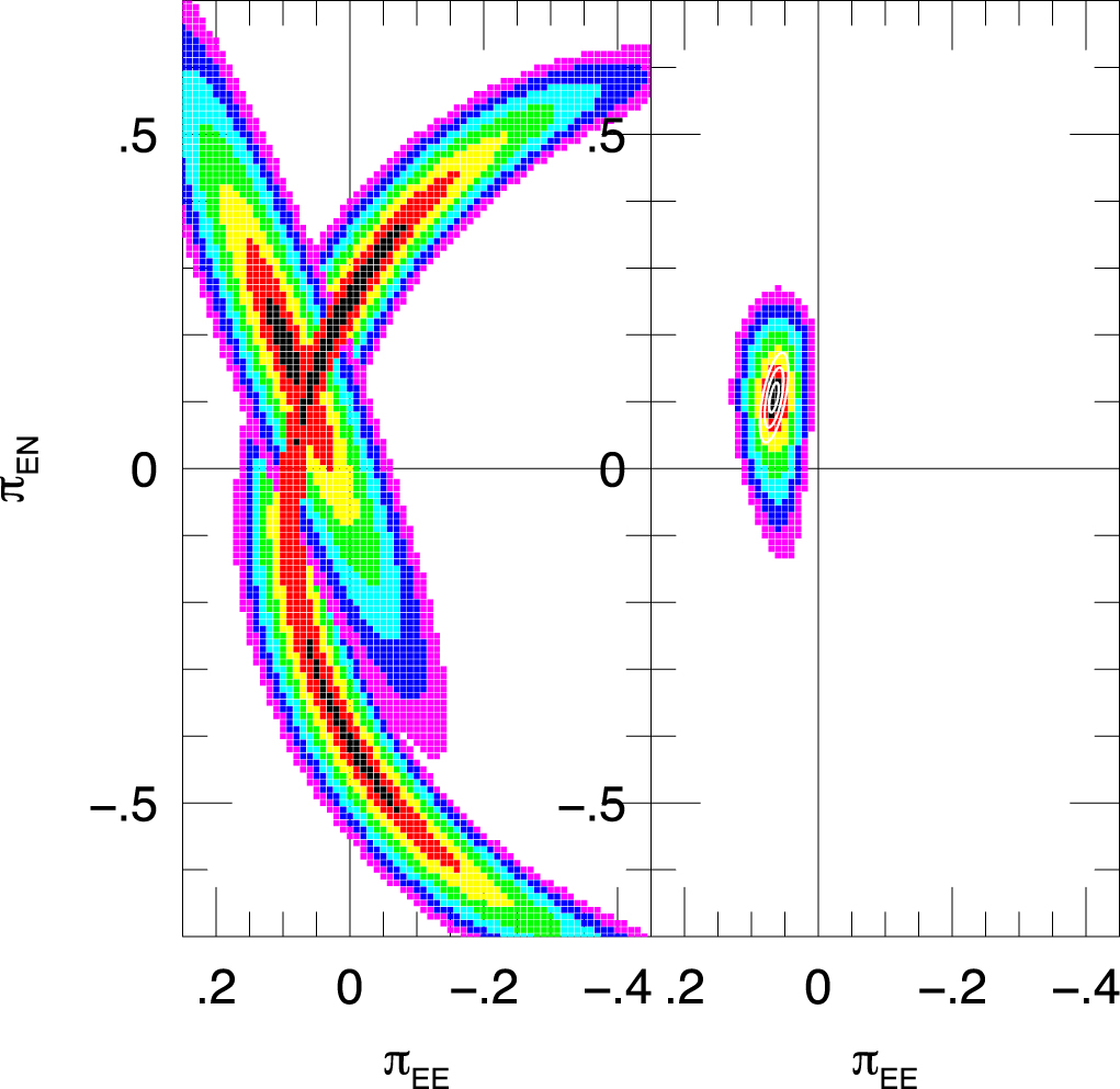
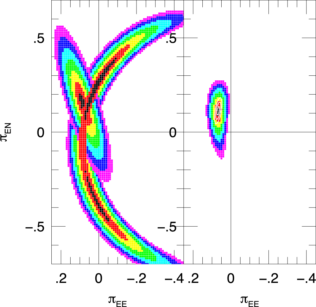
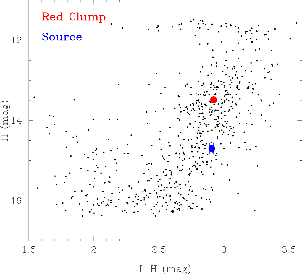
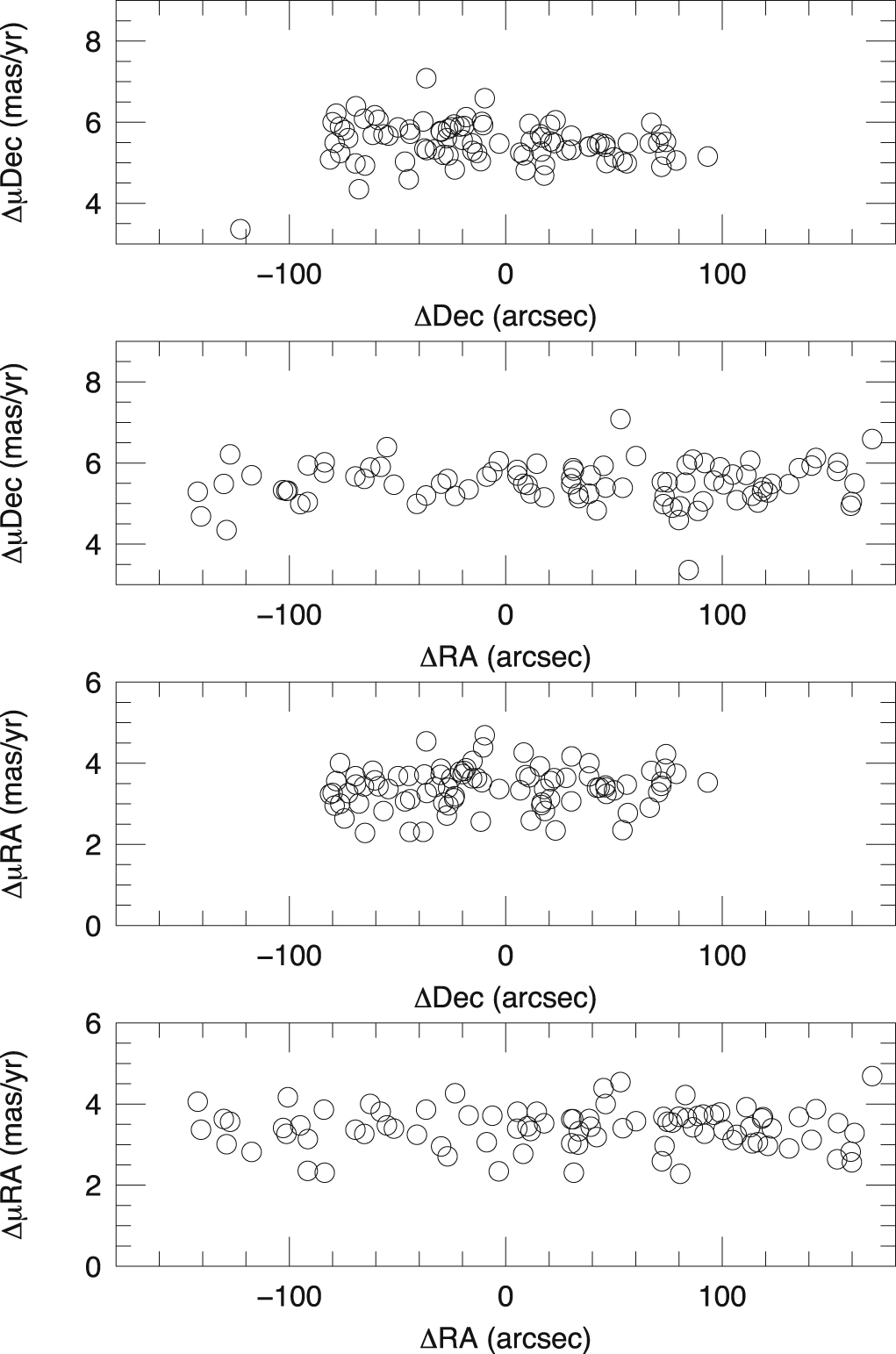
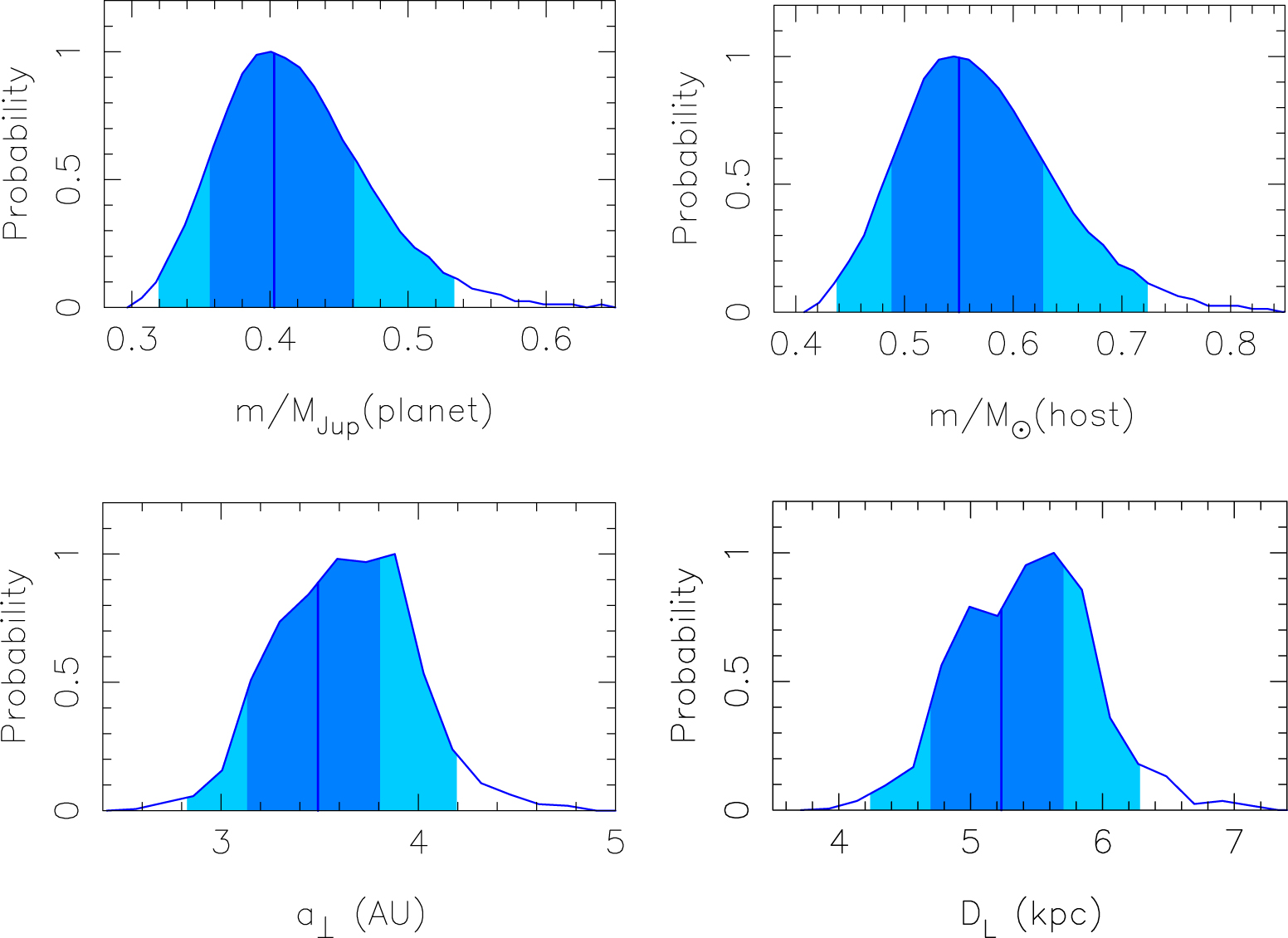
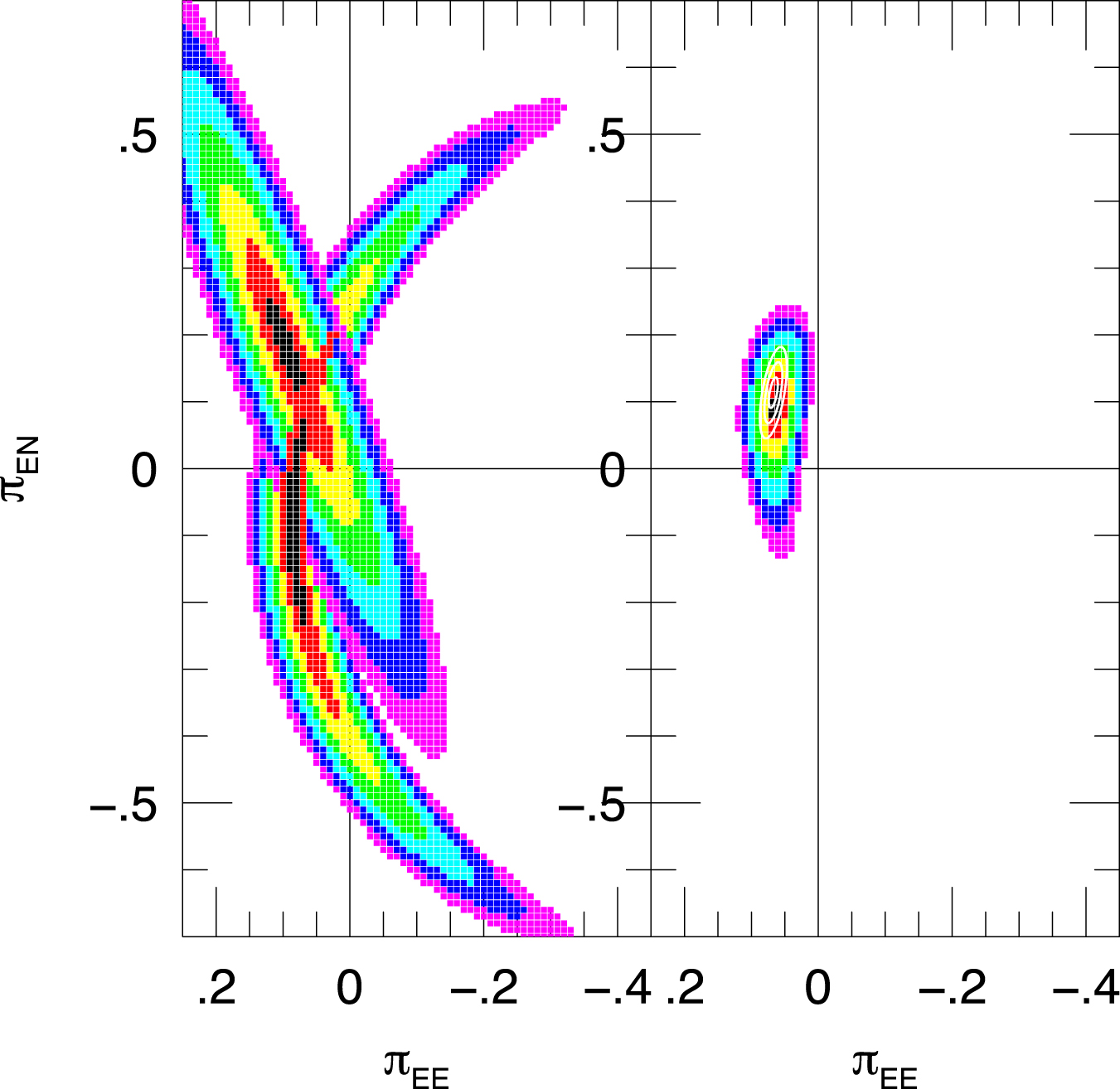