

Abstract
Salinity distribution in a large tidal estuary is subject to estuarine adjustment under the influences of multiple physical drivers such as freshwater pulses and sea level rise, and is crucial to upstream water quality, aquaculture, and ecosystem functions of the estuary. To better understand the estuarine salinity response to climate change, the unstructured-grid Finite Volume Community Ocean Model was implemented to simulate the salt intrusion in the Delaware Bay Estuary. The model was first validated by multiple observational data sets and subsequently applied in an idealized setting to examine the response of salt front to freshwater pulses in high flow conditions, followed by a long-term drought condition supported by a multi-decadal streamflow drought analysis in the estuary. The model results showed that after the freshwater pulses the salt front location moved further upstream with sea level rise. Under the simulated long-term drought condition, the adjustment timescale of salt intrusion varies nonlinearly with sea level rise. With a significant increase in sea level rise, the adjustment timescale starts to decrease. This shift suggests a transition into a different regime where the estuary becomes more stratified, as indicated by an increasing bulk Simpson number with rising sea levels.
Export citation and abstract BibTeX RIS

Original content from this work may be used under the terms of the Creative Commons Attribution 4.0 license. Any further distribution of this work must maintain attribution to the author(s) and the title of the work, journal citation and DOI.
1. Introduction
Estuaries are enclosed regions where oceanic and riverine water meet to form brackish water, with estuarine salinity varying primarily in response to tides and fresh water inputs from rivers (Geyer and MacCready 2014). Salt intrusion—the extent to which saline water penetrates upstream—in a large tidal estuary influences estuarine ecosystem functions, such as the prosperity of estuarine aquaculture (Munroe et al 2013), and the safety of public water supplies. The penetration of saline waters into the estuary is controlled by the balance between freshwater flux from the rivers and salt flux due to the tides and gravitational exchange flow, and is modulated by the meteorological forcing, bottom friction, and nonlinear interactions between topographic and bathymetric features. It remains unclear whether the contribution of each of the processes influencing salt intrusion will change in a changing climate, such as extreme drought events and sea level rise (SLR). And how the nonlinear interactions among these processes may diminish or enhance the estuarine responses is yet to be clearly understood. Recent studies (e.g. Yuan et al 2023) have shown that there has been a worldwide transition toward more frequent flash droughts that have rapid-onset from drought-free to severe drought conditions. As such, understanding the response of salt intrusion to the combined effects of flash droughts and SLR is a crucial research gap in projecting estuary conditions altered by a warmer future.
The overall goal of this study is to use a high-resolution unstructured coastal ocean model to provide insights on the estuarine responses under climate change. Within this overall goal, we have three specific objectives for this work: (1) develop an unstructured model that is capable of simulating salt intrusion in the Delaware Bay Estuary (DBE); (2) identify the main drivers that determine the salt intrusion and possible regions particularly in the upper bay that can be largely impacted by salt intrusion in changing climate; (3) quantify the adjustment timescales and its sensitivity to different processes at estuarine and shelf scales.
The rest of the paper is organized as follows. Section 2 provides the methodology including a brief description of theory, model configuration, validation, and drought analysis. Section 3 presents the model results and discusses the impact of regional climatic forcing on salt intrusion. Concluding remarks are shared in section 4.
2. Methodology
2.1. Study site
The DBE, which contains one of the longest undammed rivers in the eastern US, is a funnel-shaped estuary that extends from the narrow Delaware River channel at Trenton, NJ (River Kilometer 216) to the large lower bay connected to the Atlantic Ocean. The mean water depth in the DBE is about 7 m, with the deepest depth exceeding 45 m (figure 1). The tides in the DBE are predominantly semi-diurnal with up to 96% of the tidal variance contributed from M2 and S2 tides (Aristizábal and Chant 2013). The tidal amplitude and velocity increase upstream, with the amplitude approximately 1.5 m at the estuary entrance and the maximum tidal current approximately 1 m s−1 (Wong and Sommerfield 2009). The DBE has two main tributaries, the Delaware River and the Schuylkill River, with the former contributing over 50% of the freshwater inflow to the DBE (Whitney and Garvine 2006). The DBE is also manually connected to Chesapeake Bay through the Chesapeake & Delaware Canal (C & D Canal) at River Kilometer 94.
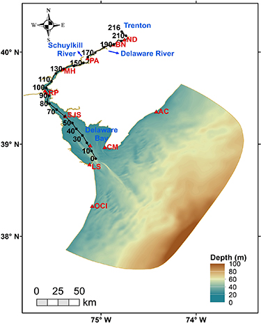
Figure 1. Model domain, geographical locations of the NOAA tide gauges (red triangle) and river kilometer system (black line) in the Delaware Bay Estuary. The tide gauges are listed (red triangle) as Atlantic City (AC), Ocean City Inlet (OCI), Cape May (CM), Lewes (LS), Brandywine Shoal Light (BSL), Ship John Shoal (SJS), Reedy Point (RP), Delaware City (DC), Marcus Hook (MH), Philadelphia (PA), Burlington (BN), and Newbold (ND). The river kilometer system is measured from the bay entrance with horizontal distance (black number) in unit of kilometer.
Download figure:
Standard image High-resolution image2.2. Streamflow drought analysis
We constructed the flow conditions for idealized experiments to approximate a rapid transition from a high flow event to an extended, historically worst drought with persistent low flow conditions. Our analysis of streamflow drought was conducted on the two main tributaries that contribute freshwater to DBE. Drought events for each tributary were identified from multi-decadal daily streamflow simulations (1982–2020; more details in the supplemental material) generated from a process-based Distributed Hydrology Soil Vegetation Model (DHSVM; Wigmosta et al 1994, Sun et al 2015).
The drought condition was analyzed by the standardized streamflow index (SSI; Nalbantis and Tsakiris 2009). We calculated SSIs on both 3-month and 6-month timescales, with very similar results for the worst drought case in both tributaries. Here we present the results based on the 3-month SSI. The worst drought event was identified as the one with the lowest SSI and the longest duration (figure 2). For the two tributaries, the most severe drought since 1980 has an SSI value of −2.2, classified as an exceptional drought according to Hao et al (2014, see table 2). The low flow level was then determined by averaging flow during the worst drought period.

Figure 2. (a) and (b) Monthly Standardized Streamflow Index (SSI) and (c) and (d) monthly streamflow for Delaware River and Schuylkill River from year 1982–2020. The dashed line at SSI = −1.3 marks the threshold for severe drought (D2), with lower SSI values indicating more severe conditions. A lower SSI suggests more severe drought. Red circles mark the worst drought since 1982 defined by the longest duration of the lowest SSI at −2.2.
Download figure:
Standard image High-resolution image2.3. Theory
The distribution of salinity in a tidal estuary is mainly a result of competition between the seaward river flow that moves the salt out of the estuary and a upstream salt transport associated with the baroclinic exchange flow and tidal motions (Hansen and Rattray Jr 1966, Monismith et al 2002, Geyer and MacCready 2014). At steady state, there is a balance between the two processes. Suppose in a tidal estuary, the tidally and cross-sectionally averaged salt balance equation can be written as follows (e.g. Monismith et al 2002)

where κx
is the dispersion coefficient in the along-channel direction (x),  is the area of local cross-section, Qr
is the river discharge, S is the salinity. At steady state and within the limit of salt flux solely provided by mechanism of gravitational circulation, the salt intrusion length XS
(the distance of the location of isohaline of salinity S measured from a reference point downstream) is proportional to
is the area of local cross-section, Qr
is the river discharge, S is the salinity. At steady state and within the limit of salt flux solely provided by mechanism of gravitational circulation, the salt intrusion length XS
(the distance of the location of isohaline of salinity S measured from a reference point downstream) is proportional to  (see Monismith et al (2002) for more detailed derivation) where the scaling with constant cross-section area gives
  (see equation (6) in Monismith et al
2002). In particular, X2, defined as the location where the 2 g kg−1 isohaline intersects the estuary bottom as measured from the bay entrance, will be used to indicate the salt intrusion length thereafter due to its significant correlation with the abundance across all trophic levels as reported by Jassby et al (1995). Empirical correlations with observational datasets suggest that this relationship could relax depending on the characteristic of the estuary. In Hudson River for instance, m is about −0.38 and −1.19 for low and high river discharge, respectively (Abood 1974). A weaker relationship was found in San Francisco Bay with
(see equation (6) in Monismith et al
2002). In particular, X2, defined as the location where the 2 g kg−1 isohaline intersects the estuary bottom as measured from the bay entrance, will be used to indicate the salt intrusion length thereafter due to its significant correlation with the abundance across all trophic levels as reported by Jassby et al (1995). Empirical correlations with observational datasets suggest that this relationship could relax depending on the characteristic of the estuary. In Hudson River for instance, m is about −0.38 and −1.19 for low and high river discharge, respectively (Abood 1974). A weaker relationship was found in San Francisco Bay with  (Monismith et al
2002). In the DBE, however, Aristizábal and Chant (2013) found that
(Monismith et al
2002). In the DBE, however, Aristizábal and Chant (2013) found that  based on the results from numerical simulations with a series of constant river discharge. Cook et al (2023) reported that m is close to −1/5 in the DBE.
The adjustment timescale, the time it takes for salinity distribution in the estuary to adjust to a new condition, can be written in an analytical format by assuming there is an abrupt change in the freshwater flux in a partially-mixed estuary with length  (Kranenburg 1986, Hetland and Geyer 2004):

where  is the salinity at the estuary entrance, and
  is the cross-sectionally averaged salinity in a steady state at a given
  . MacCready (1999) reexamined the time-dependent response of a rectangular estuary to both changes in riverine flows and mixing using a two-layer model, and reported longer adjustment timescale in intermediate depth estuaries compared to shallow and deep estuaries. Using a three-dimensional numerical model in a configuration of an idealized prismatic estuary with constant vertical mixing and steady river flow, Hetland and Geyer (2004) revisited the classic theories of estuarine circulation, and found asymmetric responses of adjustment timescale to increasing/decreasing river flows, which cannot be answered by the linear theory of Kranenburg (1986). Instead, this asymmetry was attributed to quadratic bottom drag.
These theories, based on both theoretical and empirical correlations, provide a useful framework to estimate the salt intrusion length and the associated adjustment timescale. However, these theories do not answer how salt intrusion length and adjustment timescale would change under a combination of regional climatic forcing such as long-term drought and SLR, partly due to the lacking of observations on such future projections. And we try to examine this using a three-dimensional high-resolution model that will be described in section 2.4.
2.4. Model description and configuration
The DBE model was based on the Finite Volume Community Ocean Model (FVCOM; Chen et al 2003), which has been extensively used to study the nonlinear interactions between river flow, storm surge, and tides (Xiao et al 2021), and has also been instrumental in investigating compound flooding (Deb et al 2023) and enhancing storm surge forecasts during extreme events (Liu et al 2020). The model grid used for this study is modified from those in the earlier applications to include the broad shelf outside the DBE (figure 3). It consists of 126 722 triangle elements and 68 416 nodes with 30 uniform sigma layers in the vertical direction. The resolution of the model grid ranges from 4 km on the shelf to 100 m in the DBE with the finest resolution of O(30)m in the Delaware River channel. The sea surface wind and air pressure fields are obtained from NCEP Climate Forecast System Version 2 (CFSv2) Selected Hourly Time-Series Products (Saha et al 2014). Freshwater discharge for the model validation period is prescribed at two main tributaries using the USGS stream gauge data from Delaware River at Trenton, NJ (USGS 1463500) and Schuylkill River at Philadelphia, PA (USGS 01474500). The salinity on the open ocean boundary is extracted from the HYCOM database of GOFS 3.1: 41-layer HYCOM + NCODA Global 1/12∘ Analysis (Metzger et al 2017). The tidal open boundary condition is specified with time series of surface elevations obtained from the Oregon State University TPXO global ocean tide database v9 (Egbert and Erofeeva 2002) and includes 21 tidal constituents: M2, S2, N2, K2, K1, O1, P1, Q1, MM, M4, MN4, MS4, 2N2, S1, 2Q1, J1, L2, M3, MU2, NU2, and OO1.

Figure 3. (a) Model domain in the Delaware Bay Estuary with zoom-in for (b) model grid in the river channel.
Download figure:
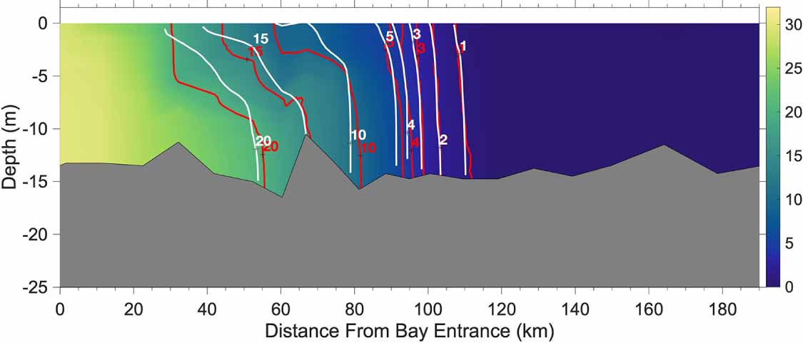
Standard image High-resolution imageThe model is evaluated based on a three year-long simulation forced by the historical meteorological forcing from year 2010 to 2012. The salinity field is initialized from the climatological salinity distribution along the river kilometer system based on the Delaware River Basin Commission monthly salinity survey from 1979 to 2016, of which the values in general increase from the bay entrance to the upper bay. Then the model is validated against multiple data sets. An example of the model comparison with the observed water level at 12 National Oceanic and Atmospheric Administration (NOAA) tidal gauges and the observed salinity transect along the River Kilometer system (black line in figure 1) during the Rutgers research voyages in June 2010 are shown in figures 4 and 5, respectively. The results show that the DBE model well reproduces the hydrodynamics, in particular, the location of the salt front (e.g. the isohaline of 2 g kg−1) which is crucial to understand the response of salt intrusion to regional climatic forcing.

Figure 4. Observed (blue) and modeled (red) water level η (in meter) at 12 NOAA tidal gauges (red triangle in figure 1) in the Delaware Bay Estuary corresponding to the survey period in figure 5. The Pearson correlation coefficient (R) and root mean square error (RMSE) are indicated at each station.
Download figure:
Standard image High-resolution image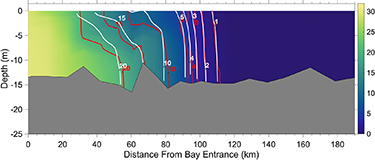
Figure 5. Observed salinity distribution (background and red) from Chant Cruise 2010 (3 June 2010–4 June 2010) along the river kilometer system shown in figure 1. The modeled salinity from FVCOM is in white.
Download figure:
Standard image High-resolution imageFollowing model validation, a series of simulations (table 1) are conducted in an idealized setting to investigate the effect of various regional climatic forcing factors, including SLR, shelf processes, and estuarine wind on salt intrusion. Because this study is mainly focused on salt intrusion into the main stem of Delaware River from the ocean boundary, in the baseline case (R1), the C & D Canal is assumed to be closed as a simplification to remove its effect. In each simulation, the model is initialized with the same low river flow condition extracted from the previously validated simulation at 28 September 2010 12:00:00 UTC (0 Day in model time). This initial condition was chosen because the salinity distribution in the river channel was in a quasi-steady state due to the low flow condition in September. A few days after this time, there was a high flow event that pushed the salt front downstream and reshuffled the estuary. Therefore it allows for the investigation on the internal characteristic of the estuarine adjustment in drought condition. The idealized river discharge is constructed to represent a quick shift from flood to drought conditions, starting with the peak flow of a high flow event observed in October 2010 (Xiao et al
2021), followed by a prolonged five-month drought condition with a persistent low river flow (figure 6), resembling the most extreme drought condition identified in section 2.2. Cases R2-R6 represent the scenarios with SLR ranging from 0.5 m to 4.0 m, in which the water elevation is uniformly augmented across the entire domain including the open boundary by assuming no shoreline retreat, i.e. keeping the channel geometry unchanged. The choice of SLR is inspired by the latest projections for relative SLR along the U.S. coastlines by Sweet et al (2022)(see their table 2.3). The salinity values on the shelf ( ) outside the DBE are reduced by 5% in Case R7 and they are increased by 5% in Case R8 compared to Case R1, which is motivated by the relative change (∼5%) in surface salinity on the Northeast Shelf over the past few decades (National Oceanic and Atmospheric Administration 2020). In particular, Case R7 represents the salinity decrease on the shelf potentially caused by southward transport of less saltier water arising from accelerated ice melting in the arctic in a warmer future, and R8 represents the salinity increase on the shelf potentially due to excess evaporation or other broader circulation shifts. The estuarine wind forcing is turned off in Case R9 to examine the effect of meteorological forcing on the salt intrusion.

Figure 6. Time series of (a) the discharge from Schuylkill River (red) and Delaware River (black) with the peak flow of a high flow condition followed by an extended extreme drought condition with the characteristics of the drought event identified in section 2.2, (b) the location of bottom salinity of 2 g kg−1 (X2) in river kilometer measured from the bay entrance, (c) Simpson number ( ; equation (6)), and its gravitational straining component (d)
  and tidal mixing component (e)
  .
.
Download figure:
Standard image High-resolution imageTable 1. Summary of simulations.
| Cases | Sea level rise (m) |

| Wind |
|---|---|---|---|
| R1 | 0.0 | 100% | On |
| R2 | 0.5 | 100% | On |
| R3 | 1.0 | 100% | On |
| R4 | 2.0 | 100% | On |
| R5 | 3.0 | 100% | On |
| R6 | 4.0 | 100% | On |
| R7 | 0.0 | 95% | On |
| R8 | 0.0 | 105% | On |
| R9 | 0.0 | 100% | Off |
3. Results
3.1. Response of salt intrusion length to regional climatic forcing
We started the analysis by examining how SLR affects salt intrusion length X2. The temporal variations of tidally averaged X2 with different SLR, shown in figure 6(b), indicate that X2 remains relatively stable for all cases with respect to the initial value ( River Kilometer 115) in the first few days of the simulation, before the discharge pulses. The river discharge at Schuylkill River increases until reaching the peak within a day, followed with a ∼12 h delay by an increase in the Delaware River discharge. The summed discharge pulses from both rivers push the salt front location downstream until it reaches a minimum
  . The minimum salt intrusion length (
 ) increases with SLR, ranging from River Kilometer 83 in the baseline case (R1) to River Kilometer 100 in the case with the highest SLR (R6). After the transient adjustment associated with the freshwater pulses, since day 17, the salt front starts to move upstream, as river flow drops to a base level during the simulated drought condition. As a result, the salt intrusion length increases until it reaches a new steady state, defined by the maximum value of X2. The maximum salt intrusion length,
  , increases with SLR, ranging from River Kilometer 127 in the baseline case (R1) to River Kilometer 152 in the highest SLR scenario (R6).
In addition to SLR, we also examined how changes in salinity on the shelf affect the salt intrusion in the DBE. The minimum and maximum of X2 is about River Kilometer 82 and River Kilometer 125 in Case R7, about River Kilometer 85 and River Kilometer 129 in Case R8, respectively, indicating only a weak effect on salinity intrusion into the Delaware Bay. The effect of estuarine wind forcing also seems to not be significant as the maximum X2 is around River Kilometer 127 when wind forcing is excluded, which is similar to that in R1 in which the wind forcing is included.
3.2. Response of adjustment timescale to regional climatic forcing
Figure 6(b) shows that different SLR cases have different adjustment timescales to equilibrium under drought conditions. To compare its variation with different scenarios, we define the adjustment timescale ( ) as an asymptotic exponential function between
  and
and  ,
,

where  is the X2 at time t with
  and
and  for the minimum and maximum value in X2, and equation (3) can be written as

which can be rewritten as

where  and α is time in days. This indicates that the steeper the slope (
 ) is, the shorter the adjustment timescale.
The adjustment timescale ( ) for different scenarios are summarized in figure 7. Note that
  varies nonlinearly with respect to SLR (table 2). Adjustment timescale was primarily influenced by SLR. The changes in the shelf salinity did not significantly affect the adjustment timescale, whereas
  was 40 and 39 day when salinity reduced/increased by 5%, respectively. Also, without estuarine wind forcing,
  in R9 decreased by 5 day compared to the baseline case.

Figure 7. The adjustment timescale ( ) under different climatic forcing with
  , where α is the relative time (in days) to the one at which
  , and
, and  ).
).
Download figure:
Standard image High-resolution imageTable 2. Summary of adjustment timescale  (day).
| R1 | R2 | R3 | R4 | R5 | R6 | R7 | R8 | R9 | |
|---|---|---|---|---|---|---|---|---|---|
 (day) (day) | 39 | 40 | 48 | 44 | 35 | 26 | 40 | 39 | 34 |
Figure 7 indicates that  tends to first increase with SLR, then after 1 m SLR it starts to decrease. This suggests that there is a regime shift in the estuarine flow with increasing SLR. To address this question, we compared the adjustment timescale,
  to the Simpson number,

a ratio of potential energy increases due to gravitational straining, and decreases due to tidal mixing (Stacey and Ralston 2005, Burchard and Hetland 2010, Geyer and MacCready 2014), where  is along-channel buoyancy gradient, Cd
is bottom drag coefficient, Ut
is tidal velocity, and H is water depth, g is gravitation acceleration, ρ0 is reference density, γ is haline expansion coefficient, and
is along-channel buoyancy gradient, Cd
is bottom drag coefficient, Ut
is tidal velocity, and H is water depth, g is gravitation acceleration, ρ0 is reference density, γ is haline expansion coefficient, and  is along-channel salinity gradient. Here Si is averaged over a control volume with lateral boundary bounded by River Kilometer 65 and X2. Si > 1 indicates gravitational circulation dominates and the estuary tends toward more stratified, and values much smaller than one indicate mixing dominates and the estuary tends toward well-mixed.
The time series of Si, shown in figure 6(c), shows that the magnitude of Si increases with SLR, particularly between 20 and 50 day in the simulation time when the salt front starts to move upstream to its new equilibrium position. The variation of  with respect to the time averaged Simpson number
  and SLR, presented in figure 8, shows that
  tends to be separated into two regimes where
  grows until capped by the limit under low SLR and starts to fall under high SLR, while
  keeps increasing with SLR, consistent with trend of the freshwater residence time which increases with SLR as well (not shown). Since the larger
  indicates that the advection of horizontal salinity gradient becomes dominant over the tidal mixing through the water column, the result suggests that for SLR greater than 1 m, it enters a different regime where the estuary flow gets more stratified and less well mixed under drought conditions.

Figure 8. Effects of sea level rise on the adjustment timescale ( ) and time-averaged Simpson number
  .
.
Download figure:
Standard image High-resolution imageIn fact, the role of SLR on  and salt intrusion can be seen by comparing the evolution of each component in
  (figures 6(d) and (e)) as H increases with increasing SLR. Numerator
  increases with higher SLR (e.g. between 20 and 50 simulation day) whereas denominator
  decreases with higher SLR. Both contribute to a larger
  . In other words, there will be positive feedback from both horizontal advection and tidal mixing on
  .
.
The adjustment timescale,  , is inversely proportional to the estuarine circulation,
  . The estuarine circulation, ue
, can be scaled as
. The estuarine circulation, ue
, can be scaled as

where ν is (constant) viscosity (Hansen and Rattray Jr 1966, Hetland and Geyer 2004). That is, the estuarine circulation increases with increasing baroclinicity ( ), and decreases with increasing drag (
 ), the same tendencies represented in the Simpson number (Si).
The two dynamical regimes can be explained by understanding the shift in the tidal dynamics, which do not have a linear response to SLR throughout the Bay. For SLR up to 1 m, increasing sea level increases the magnitude of the tidal currents linearly with SLR. In this case, the drag associated with the increasing tidal currents increases faster than the increase in baroclinicity caused by the increased water depth, with the net effect of reducing the estuarine circulation. Therefore  increases with SLR in this case. However, for SLR of 1 m and greater, the magnitude of the tidal currents, and hence also the associated drag, is roughly constant. This is most likely because the location of the primary integrated drag on the tidal wave propagating up the estuary has shifted upstream to shallower areas (figure 9, note that the rapid changes from positive to negative values and vice versa between 90 and 150 km occur where there are river islands, meander, or confluence in the channel, highlighting the role of local topography and bathymetry in altering the circulation), upstream of the area with strong salinity gradients. Now, increasing water depth increases the baroclinicity of the circulation with no compensating increase in drag, so the net response is that the estuarine circulation increases. Therefore
  decreases with SLR in this case.

Figure 9. The differences in time averaged  from day 20 to day 50 along river kilometer system (subtracting the values in the baseline case from each SLR case). X2 at day 20 and day 50 are denoted with dotted and dashed line, respectively.
Download figure:
Standard image High-resolution image
One weakness of this approach is that we do not consider that the inundated area associated with SLR will increase. In other words, we assume that the human response to SLR is to build coastal walls to maintain the position of the present day coastline. While this assumption is reasonable for populated regions, it may not be true for coastal marsh regions. Different mitigation strategies to coastal defense may alter tides in different ways than our model predicts, thus change the point at which SLR alters the fundamental balance of the Bay and the response to drought. However, we believe that, generally, our result that it is possible for SLR to alter Bay response to drought in ways that are not just extrapolations of present day dynamical balances—or just generally alter the response timescale of the Bay to changing freshwater forcing—is robust, even though the details will heavily depend on local Bay geometry and human response to SLR.
4. Conclusions
In this study we applied a high-resolution unstructured model based on FVCOM to investigate how regional climatic forcing could affect salt intrusion in a tidal estuary, in particular, how salt intrusion length and adjustment timescale respond to a long-term drought condition with SLR, shelf processes, and estuarine wind forcing.
The salt intrusion length reduces dramatically following the freshwater pulses in the high flow condition, and after the estuarine adjustment it increases until reaches a new equilibrium state in the drought condition. The final location of the salt front at the bottom is located more upstream with higher SLR, with an increase of about 20% in the highest SLR scenario compared to baseline.
Under the simulated drought condition, the adjustment timescale of salt intrusion varies nonlinearly with SLR. With much higher SLR, the adjustment timescale starts to decrease as it shifts into a different regime where the estuary becomes more stratified, as indicated by an increasing bulk Simpson number with SLR. This regime shift is likely due to the nonlinear response of bottom drag, that only linearly increases for SLR up to about 1 m, and baroclinicity associated with the estuarine circulation to SLR, that increases linearly with SLR for the entire range of SLR explored.
Shelf processes (i.e. open boundary salinity) and estuarine wind forcing have less significant influences on altering the salt intrusion length in the river channel compared to higher SLR. Estuarine wind forcing could increase the adjustment timescale by about 15% under the simulated drought condition. Our results suggest the influence from shelf processes on the adjustment timescale is minimal.
The analyses from this study can be applied to other partially-mixed estuaries, and provide insights for potential decision making for climate adaptation and management of salt intrusion in estuaries. There are a few interesting directions for future research that require more collaborative efforts in the modeling community. For instance, tidal marshes in the lower bay were not taken into account in this study, when included, the drag due to the vegetations on the marshes could damp the tidal amplitude, which would future alter the salt intrusion length. In addition, the modulation due to the channel flow through C & D Canal was not considered in this study. If considered, the canal could act as a mediator of the salt front location, and its contribution depends on the river discharge in the upper Delaware Bay, tides, and flow rate and salinity variation coming from the Chesapeake Bay in the canal. A joint modeling effort that connects the Delaware and Chesapeake Bay and also covers large watershed in the upper bay would be beneficial for studying salt intrusion under changing climate. Last but not least, implementing the coastal models by leveraging the output downscaled from the Earth system model such as Energy Exascale Earth System Model (E3SM) could be useful to examine the joint effect and uncertainty of different natural and human processes on various temporal and spatial scales including extreme events and future climate projections.
Acknowledgments
This work was supported by the Earth System Model Development and Regional and Global Modeling and Analysis program areas of the U.S. Department of Energy, Office of Science, Office of Biological and Environmental Research as part of the multi-program, collaborative Integrated Coastal Modeling (ICoM) project. All model simulations were performed using resources (Constance) available through Research Computing at Pacific Northwest National Laboratory (PNNL). PNNL is operated by Battelle Memorial Institute for the U.S. Department of Energy.
We thank John Wilkin and Robert J Chant for sharing the salinity data from Rutgers research voyages for model validation. We also appreciate Parker MacCready for the insightful discussion. Discussions with Fanghui Chen and Salme E Cook during early stage of this study are much appreciated. Special thanks to two anonymous reviewers for their significant contributions in enhancing the manuscript.
Data availability statement
The data that support the findings of this study are openly available at the following URL/DOI: https://doi.org/10.25584/2335335. Data will be available from 30 June 2024.
Supplementary data (0.7 MB PDF)