

Abstract
The Large Array Survey Telescope (LAST) is a wide-field visible-light telescope array designed to explore the variable and transient sky with a high cadence. LAST will be composed of 48, 28 cm f/2.2 telescopes (32 already installed) equipped with full-frame backside-illuminated cooled CMOS detectors. Each telescope provides a field of view (FoV) of 7.4 deg2 with 1 25 pix−1, while the system FoV is 355 deg2 in 2.9 Gpix. The total collecting area of LAST, with 48 telescopes, is equivalent to a 1.9 m telescope. The cost-effectiveness of the system (i.e., probed volume of space per unit time per unit cost) is about an order of magnitude higher than most existing and under-construction sky surveys. The telescopes are mounted on 12 separate mounts, each carrying four telescopes. This provides significant flexibility in operating the system. The first LAST system is under construction in the Israeli Negev Desert, with 32 telescopes already deployed. We present the system overview and performances based on the system commissioning data. The Bp 5σ limiting magnitude of a single 28 cm telescope is about 19.6 (21.0), in 20 s (20 × 20 s). Astrometric two-axes precision (rms) at the bright-end is about 60 (30) mas in 20 s (20 × 20 s), while absolute photometric calibration, relative to GAIA, provides ∼10 millimag accuracy. Relative photometric precision, in a single 20 s (320 s) image, at the bright-end measured over a timescale of about 60 minutes is about 3 (1) millimag. We discuss the system science goals, data pipelines, and the observatory control system in companion publications.
Export citation and abstract BibTeX RIS

Original content from this work may be used under the terms of the Creative Commons Attribution 3.0 licence. Any further distribution of this work must maintain attribution to the author(s) and the title of the work, journal citation and DOI.
1. Introduction
Scanning the sky repeatedly has revealed intriguing facts about the physical Universe. From the detection of the Earth's precession by Hipparchus, to the discovery of the proper motion of stars by Halley, and the extragalactic novae of Fritz Zwicky. With the advance of technology, sky surveys have made great progress in the past 20 years. Sky surveys revealed new kinds of exploding phenomena like super-luminous supernovae (Quimby et al. 2007; Quimby et al. 2011), discovered thousands of exoplanets around distant stars (e.g., Zhu & Dong 2021), measured the distances to a large number of stars (e.g., Gaia Collaboration et al. 2016), and identified the majority of Near Earth Objects larger than 1 km.
While sky-surveys like the Zwicky Transient Facility (ZTF; Bellm et al. 2019), Pan-STARRS (Chambers et al. 2016), ASAS-SN (Kochanek et al. 2017), and ATLAS (Heinze et al. 2018) provide excellent monitoring of the sky, making progress in our understanding of the Universe requires pushing toward observing a larger fraction of the sky continuously (i.e., around the globe) at high cadences. Furthermore, it is desirable to increase the cost-effectiveness of survey telescopes, otherwise, in the future, it will be expensive and difficult to surpass the performances of the Large Survey of Space and Time (LSST; LSST Science Collaboration et al. 2009; Ivezić et al. 2019). Here, following Ofek & Ben-Ami (2020), we define the cost-effectiveness of a transient's survey telescope as the relative volume of the Universe that can be observed by a system per unit time per unit cost (i.e., grasp per unit cost). Ofek & Ben-Ami (2020) argued that with the availability of affordable back-side-illuminated CMOS detectors with small pixels (smaller than about 4 μm), and taking advantage of the affordability of off-the-shelf components, it has only now become significantly more cost-effective to construct survey telescopes composed of multiple small telescopes, compared with a single large telescope with the same grasp (relative volume per unit of time). In fact, the increase of small telescope cost-effectiveness is so pronounced, we believe that, with current technology, there is no point in building telescopes larger than about 0.5 m for seeing-limited visible-light imaging purposes. Another future project that has the potential to demonstrate this point is the Argus array (Law et al. 2022).
Following these lines of argument, we are constructing the first system (also referred to as a node) of a new cost-effective survey telescope: the Large Array Survey Telescope 9 (LAST). LAST is currently the sky survey system with the highest grasp (Figure 1). In the near future, both LSST (Ivezić et al. 2019) and ULTRASAT (Sagiv et al. 2014, Y. Shvartzvald et al. 2023, in preparation) will surpass this grasp. Nevertheless, the LAST geographic position elevates our capabilities in terms of monitoring the sky around the globe. We estimate that the cost-effectiveness of LAST is about an order of magnitude higher compared to most other survey telescopes.

Figure 1. The grasp (relative volume per unit time) of several sky surveys, as a function of wavelength, as calculated using the used or planned survey exposure time, and published limiting magnitudes (rather than aperture, seeing, and sky brightness). The plot is calculated for a source with 20,000 K blackbody spectrum (e.g., hot transient). The plot also takes into account the on-sky fraction of time (about 0.25 for a typical ground-based observatory), and the survey exposure time and dead time (if available). The y-axis is in arbitrary units, normalized such that the LAST grasp is about 1. LAST 48, assumes a LAST node with 48 telescopes, and sky brightness of 21.0 mag arcsec2. Black-GEM ×4, assumes four Black-GEM telescopes (Bloemen et al. 2015), GOTO ×8 assumes the GOTO system with eight telescopes (Steeghs et al. 2022), for ATLAS we assume two telescopes (Tonry 2011), while MASTER is calculated assuming seven sites. The Argus array-like project (Law et al. 2022) has the potential to be at the level of LSST to about an order of magnitude above LSST. However, we do not know the exact expected parameters for this system.
Download figure:
Standard image High-resolution imageHere we describe the LAST system, design, strategy, and preliminary performances. In companion papers, we discuss the LAST science goals (Ben-Ami et al. 2023), pipeline (Ofek et al. 2023, hereafter pipeline paper), and observatory control (E. Segre et al. 2023, in preparation). The first science results from LAST, including analysis of the DART (Rivkin et al. 2020) impact observations, are described in E. O. Ofek et al. 2023, in preparation.
In Section 2, we provide an overview of the system, while in Section 3 we discuss data rate considerations that dictate the survey and pipeline strategy. In Section 2.4, we discuss the survey strategy, and in Section 5 we provide an overview of the system software. In Section 6, we describe the measured camera properties, while in Section 7 we present some of the system's initial performances. Future follow-up facilities to support LAST are discussed in Section 9, and we conclude in Section 10.
2. LAST System Overall Description
LAST is designed to be a cost-effective, modular, and extendable survey telescope. A full LAST node is composed of 48 (=Ntel), 28 cm telescopes under a single rolling-roof structure. Each telescope (Section 2.3) is equipped with a full frame (i.e., 36 × 24 mm-size) backside illuminated and cooled CMOS detector (Section 2.5). A group of four telescopes are mounted on a single, two-sided, German Equatorial mount (see Section 2.4). Each sub-system of four telescopes is controlled by two 30-core 256 GB RAM computers (see Section 2.7). In addition, these computers are responsible for running the image processing pipeline (Section 5.1; Ofek et al. 2023).
A summary of a LAST node system parameters are provided in Table 1.
Table 1. The First LAST Node System's Parameters
| Property | Value |
|---|---|
| Number of telescopes (planned; 2023 June) | 48 |
| Number of telescopes (2023 March) | 32 |
| Telescopes per mount | 4 |
| Telescope aperture | 279.4 mm |
| System equivalent aperture | 1.9 m ( ) ) |
| Telescope focal length | 620 mm |
| Pixel scale | 125 pix−1
|
| Telescope FoV | 2.2 × 3.3 deg ≅7.4 deg2 |
| System FoV | 355 deg2 |
| Total number of pixels | ≅2.9 × 10⁹ |
| Bp Limiting magnitude (5σ in 20 s) | ≈19.6 mag |
| Bp Limiting magnitude (5σ in 20 × 20 s) | ≈21.0 mag |
| Location | Neot-Smadar, Israel |
| Longitude (WGS84) | 35.0407331deg E |
| Latitude (WGS84) | 30.0529838deg N |
| Height (WGS84) | 415 m |
Note. Limiting magnitude is estimated during dark time, and airmass of about 1, sky brightness of 21.0 mag arcsec2, image quality of ≈28, for sources with color of Bp − Rp = 1.0 mag near the field center (see Section 7.3 for details).
Download table as: ASCIITypeset image
In Figure 1, we present the estimated grasp, as a function of wavelength, for several survey telescopes for which the system parameters are known to us. The total hardware and construction costs for a LAST node is $1.5M. This includes all the telescopes, cameras, mounts, computers, communication, and construction costs including the enclosure, and site infrastructure. The man-power cost for the system development (software and hardware) is estimated at about $500k. The LAST PIs are Eran Ofek & Sagi Ben-Ami.
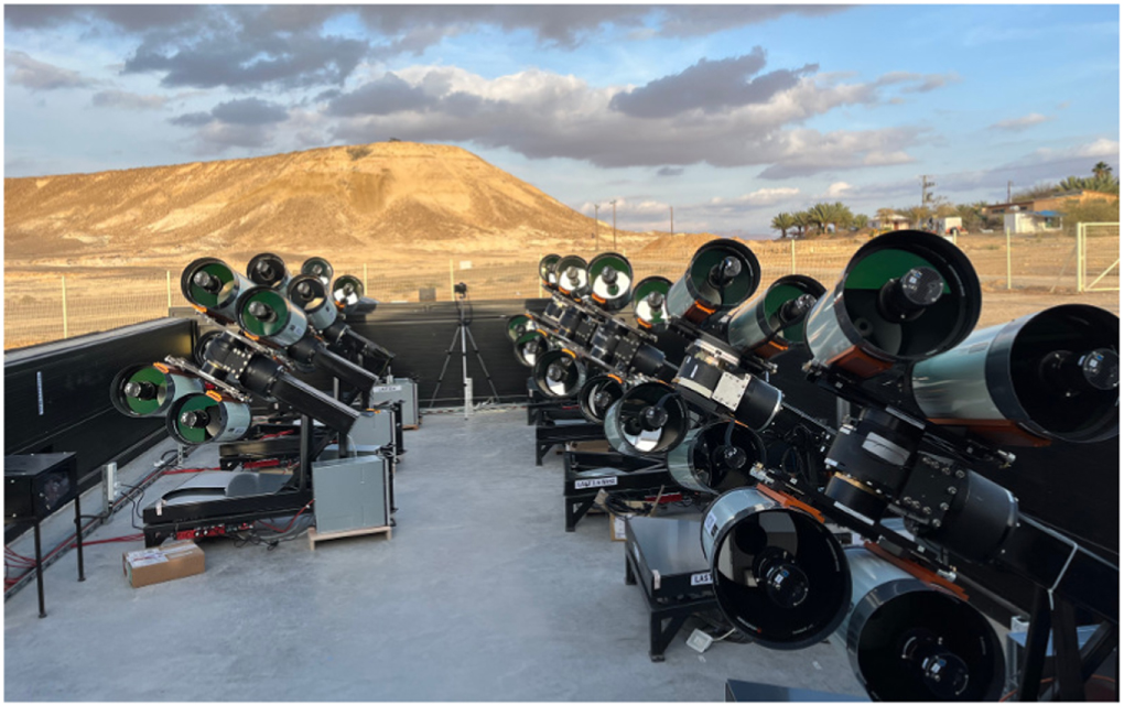
The LAST system is highly modular, both in terms of hardware and software. This modularity as well as the relatively small physical size of the components makes the system flexible, but it also makes it easy to extend, deploy, and maintain. Almost all the components (with the exception of the enclosure and mounts) are off-the-shelf products that are manufactured in large numbers. Figure 2 shows an image of the first LAST node with 32 telescopes, in Neot-Smadar.

Figure 2. LAST with 32 telescopes installed. The enclosure is fully open.
Download figure:
Standard image High-resolution image2.1. Site
The sky brightness in the Neot-Smadar site is relatively poor. In the past two years the V-band sky brightness degraded from about 21.0 mag arcsec−2 to about 20.6 mag arcsec−2. A major consideration for the site selection was the speed at which the observatory can be built in the site (e.g., permits). We note that building LAST in a dark site on Earth (i.e., 22 mag arcsec−2), may improve the system limiting magnitude by about 0.7 mag.
Although LAST is marginally seeing-limited, we are planning to use this site for additional telescopes (Section 9), and therefore we have measured the site seeing extensively. The seeing was mainly measured using a Cyclope
10
seeing monitor device. The site mode, median, and mean seeing measured over 180 nights is about 13, 14, and 15, respectively. The histogram of all seeing measurements is shown in Figure 3.

Figure 3. Histogram of about 75,000 seeing measurements taken over 180 nights prior to the observatory construction. The mode, median, and mean seeing measured over 180 nights is about 13, 14, and 15, respectively. The lower and upper 5% percentile of the measurements is 098 and 236, respectively.
Download figure:
Standard image High-resolution image2.2. Enclosure
The LAST enclosure is a custom-made rolling-roof structure. The inner usable size of the structure is 5.2 m by 11 m. The roof is composed of three parts that move in the direction of the long axis of the structure. When the roof is open, the structure walls are 1.2 m high, with the exception of the enclosure entrance. The structure has additional upward/downward-moving walls on three sides (South, East and North). These walls can go up in order to block strong winds. The LAST enclosure was designed to be an affordable structure. The construction of the enclosure on site took about six days.
2.3. Telescopes
The LAST telescopes are Celestron ® 11-inch f/2.2 (focal length 620mm) Rowe-Ackermann-Schmidt telescopes. The telescopes' optical elements include an aspheric corrector, spherical mirror and a four-elements field flattener, and are designed to produce image quality of about 16 over the field of view of a full-frame sized camera.
Similar telescopes are also available in an 8-inch 11 and 14-inch version. In terms of grasp or etendue cost-effectiveness, and given the image quality delivered by these telescopes, the 11-inch version provides the best performance. Even if we ignore the price aspect, assuming a constant-size detector, the grasp of a single 11-inch telescope is about 35% larger than that of the 14-inch telescope.
2.4. Mounts
We use the Xerxes equatorial mount. This mount uses two direct-drive Kollmorgen ® motors that can produce torques of 60 N-m, and 33 N-m, for the hour angle and decl., respectively. The motors are equipped with Renishaw ® encoders and are controlled by two Copley ® controllers. The controllers are commanded via a serial link with an interface developed by our group. The mounts can move at a very high speed, but for safety reasons, we limit their operations to speeds of up to 12 deg s−1.
2.5. Cameras
In the focal plane of each telescope, we use the QHY600-PH camera, hosting a cooled SONY® IMX455 backside-illuminated CMOS detector. The camera and detector properties are summarized in Tables 2 and 4. In terms of Gain and Readout noise, the detector has several modes, and it is possible to control its gain and offset (bias level). We choose to work with the 16 bit mode, with a specific gain/offsets, which are listed in Table 4 (see Section 6.2).
Table 2. QHY600M-PH Camera
| Property | Value |
|---|---|
| Model | QHY600M-PH |
| Sensor | IMX455 |
| Size | 36 × 24 mm |
| Pixel size | 3.67μm |
| Pixels | 60.8 × 10⁶ |
| Sensitive pixels | 6354 × 9576 |
| Cooling | Two stage thermoelectric |
| Readout time (buffer to memory) | ≈0.7 s |
| Readout mode | Rolling shutter |
Note. The QHY600M-PH camera properties. Additional parameters are listed in Table 4.
Download table as: ASCIITypeset image
The camera uses a rolling shutter and hence can be read continuously, with negligible dead time between exposures (video mode). In the video mode, it takes about 0.7 s to read the image from the camera to the computer memory, and an additional ∼1.5 s to write the image to a spinning hard drive. Therefore, in continuous observing mode, exposures as short as 0.8 s can be used. We are currently developing an option to write images using file mapping. This may expedite the image writing process considerably.
The LAST cameras can be equipped with a single non-exchangeable filter. Indeed we are planning to test the use of such filters and polarimetry filters in the future. However, currently, we do not equip the cameras with any filters 12 . The reasoning for this is that LAST is designed to be a discovery machine, while followup (multi-band imaging and spectroscopy) will be conducted using other telescopes (see Section 9).
With the LAST telescope, the camera provides a plate scale of 125 pix, and a field of view of 3 3 × 22 (≅7.38 deg2). By default the telescopes and cameras, on each mount, are set to observe a contiguous ≈6.5 × 4.3 deg field of view. The cameras are set to have about 10' overlap, with about 3' accuracy. A set of shims allow us to switch between the open mode (i.e., wide field default), and the narrow mode (all four telescopes are pointing to the same direction). The alignment of narrow and open modes is done once on sky using a special analysis function we have developed. This process takes about 1 hr per mount. After this process is done, it takes about 10 minutes per mount to switch between open and narrow mode. All the cameras are aligned such that their long-axis is oriented North-South
13
to an accuracy of about 1°.
3 × 22 (≅7.38 deg2). By default the telescopes and cameras, on each mount, are set to observe a contiguous ≈6.5 × 4.3 deg field of view. The cameras are set to have about 10' overlap, with about 3' accuracy. A set of shims allow us to switch between the open mode (i.e., wide field default), and the narrow mode (all four telescopes are pointing to the same direction). The alignment of narrow and open modes is done once on sky using a special analysis function we have developed. This process takes about 1 hr per mount. After this process is done, it takes about 10 minutes per mount to switch between open and narrow mode. All the cameras are aligned such that their long-axis is oriented North-South
13
to an accuracy of about 1°.
The cameras are controlled using the QHY software development kit (SDK), using custom software developed by our group. This software, as well as the observatory control system, is described in E. Segre et al. 2023, in preparation.
2.6. Focusers
Each telescope is equipped with a Celestron electric focuser. The focusers are connected to the operating computer via USB links. However, to increase reliability, a new focuser system is being designed. The telescopes are focused by minimizing the width of the point-spread function (PSF) of a large number of high S/N stars near the center of the field. This is done, once, in the beginning of each night (see Section 5.4.2). However, since the focus is temperature dependent, we need to refocus the telescope during the night. This refocusing is done using a simple temperature-focus model, and this is activated, if the mount temperature varies by more than 1° Celsius.
2.7. Computers
A LAST node includes two computers per mount, plus a single control/manager computer per node. The two computers per mount are responsible for image processing (Section 5.1), controlling the mount (one of the computers), and controlling the cameras and focusers (two cameras/focusers per computer). All the computers are running Linux Ubuntu. Since all the computers should be identical in setup and software installation, we have developed a custom software installation tool (last-tool) written in bash. The tool is responsible for checking and enforcing the software policy on all computers.
Each computer has 30 cores with 256 GB RAM. In addition, each computer has a 256 GB SSD disk, 6 TB disk for software and catsHTM catalogs (Soumagnac & Ofek 2018), and two removable 14 TB disks for imaging data. Most of the CPUs are used by the image analysis pipeline.
The observatory manager computer is responsible for running the scheduler, and allocating targets to the individual mounts. This computer also controls the dome, weather stations, and auxiliary equipment. The computers are connected via a local network (1–10 Gbit s−1), that is by itself connected to the internet using a 500 Mbit s−1 fiber link.
2.8. Auxiliary Sensors
LAST is equipped with several auxiliary sensors. First, each mount has its own temperature sensor. The temperature sensor is located on the mount, near the telescopes, and its primary goal is to provide temperature readings for the focuser system (see Section 2.6).
Next, the main observatory control computer is connected to several meteorological and all-sky camera sensors, that are used by the observatory control system to determine when it is safe.
3. Data Rate Considerations
A major consideration for the LAST observing strategy and pipeline design is related to the system data rate. Each LAST camera produces a 16-bit 61 Mpix image. Due to the requirements of several science goals (e.g., exoplanets around white dwarfs; see Ben-Ami et al. 2023), we choose a nominal exposure time of 20 s. This is roughly half the expected duration of an exoplanet transiting a white dwarf. Furthermore, in our system and site, the transition
14
from readnoise dominated noise to background-dominated noise takes place at exposure times of about 5 s. With our nominal exposure time, we are in the background-dominated noise regime. Therefore, image coaddition does not suffer from significant losses. For example, by combining 20 images we gain 1.4 mag instead of 1.6 mag (i.e.,  ) improvement in limiting magnitude.
This exposure time results in a data rate of 65 Mbit s−1 per camera and 2.2 Gbit s−1 for the entire array during operations, taking into account the telescope-mount slew time and restarting the video mode at the beginning of each visit. This data rate is relatively high. 15 Such a data rate is expected to generate about 2 PB yr−1 of raw images. Given the costs associated with storing and transferring such a large amount of data, we choose a strategy that will allow us, on one hand, to reduce (if needed) the amount of stored data, and on the other hand to keep the high cadence temporal information. This high data rate also means that it is desirable to perform most of the data processing on-site.
Our default strategy is to analyze the data from each telescope separately, and let each telescope observe each field for 20 × 20 s (=400 s). Among the advantages of our 20-images per field strategy are: the ability to screen satellite glints in a single visit (Corbett et al. 2020; Nir et al. 2020; Nir et al. 2021b), and to detect main belt asteroids using their motion in about 6 min (see Ofek et al. 2023). Furthermore, for short-timescale phenomena like exoplanets around white dwarfs and flaring stars, a single visit provides a light curve of these events.
In the long-term archive, we keep only the individual image catalogs, and the coadd images (as well as other data products based on the coadded image, e.g., catalogs and subtraction images). However, the individual raw images are stored locally (on-site) in a cyclic buffer for a period of about 60 days.
This strategy allows us to reduce the data rate by a factor of about 8, but keep some of the high cadence information. In addition, if needed, the individual images can be saved from deletion. In the future we may also save the individual raw images.
4. Observing Strategy
The multi-mount, multi-telescope structure of LAST offers great flexibility in terms of operations. One question is whether to use the wide mode (28 cm telescope with 355 deg2), or a narrow mode (e.g., 1.9 m telescope with 7.4 deg2). In terms of grasp, operating the LAST system in the wide mode provides a grasp that is about 2.6 (=  ) times larger compared with the grasp of the system operated at the narrow mode. Therefore, our primary strategy is to use the wide mode, and to set the default pointing of four telescopes on each mount to cover a wide but contiguous field of view. However, for some specific science cases, the narrow mode has advantages (e.g., precision photometry; see Ben-Ami et al. 2023).
The LAST observing strategy is flexible and likely to change based on specific science goals, and capabilities. Our observing strategy can be roughly divided between three programs: (i) high cadence; (ii) low cadence; and (iii) target of opportunity (ToO). In the following discussion, we are going to assume that the ToO program will take about 5% of the observing time and that on average (all year) we have 6 hr of clear sky every night. Assuming a visit of 20 × 20 s our scanning speed is about 1470 deg2 per mount (four telescopes) per night (6 hr). This number is 17,640 deg2 per array (12 mounts). Assuming a visit of 5 × 20 s our scanning speed is about 4900 deg2 per mount per night, or 58,800 deg2 per array. The latter visit duration, therefore, allows us to scan about 9800deg2 hr−1 down to a limiting magnitude of about 20.3 on each visit.
For several reasons including science goals and pipeline performance, in the first six months of the project, we are likely to implement the 20 × 20 s visits, with a slow+fast cadence survey strategy. In this strategy, we will use 1/3 of the telescopes to observe about 5900 deg2 twice a night every two nights and about 1470 deg2 eight times per night, every night. Later on, we will consider using the 5 × 20 s visits, and cover about 104 deg2 every hour. The ToO time will be used to respond to GW, neutrinos, and GRB triggers (e.g., Abbott et al. 2017; Icecube Collaboration et al. 2017). ToOs interrupt the main program for all or some of the mounts as needed.
5. Software
The LAST project required major software efforts. These include, the pipeline (Section 5.1); the observatory control system (Section 5.2); the scheduler (Section 5.3); and apparatus calibration software (Section 5.4). Additional software tools include last-tool—a software package to enforce the LAST software installation policy on all the LAST computers.
5.1. Pipeline
The LAST data reduction pipeline is described in Ofek et al. (2023). Here we provide a brief overview of the pipeline. The on-site operations include: a basic calibration (e.g., dark subtraction, flat correction, bit-mask production), background estimation, source detection, astrometry, photometric calibration, matching sources in all the exposures from a visit, searching for variable sources (flares/transits), and searching for moving sources. The visit exposures are then registered and coadded. Next, for each coadded image, we estimate the background and variance, propagate the mask images, find and measure sources including PSF photometry, refine the astrometry, and match the sources against external catalogs. Next, the coadd images are transferred to the Weizmann Institute campus, via the internet, and image subtraction and transient detection is performed using the Zackay et al. (2016) algorithm. Reference images are built using the proper coaddition algorithm (Zackay & Ofek 2017a; Zackay & Ofek 2017b).
In order to reduce costs and complexity it was critical to reduce the amount of computing (and electricity) power on site. Using off-the-shelf software packages will require an order of magnitude increase in the amount of computing power on site. Therefore, we have developed a new efficient image processing code for LAST and ULTRASAT (Sagiv et al. 2014, Y. Shvartzvald et al. 2023). For example, our source extraction code which performs source finding and PSF photometry is about a factor of 30 faster than SExtractor (Bertin & Arnouts 1996). The code is based on the tools developed in Ofek (2014), Soumagnac & Ofek (2018), Ofek (2019), and is available via GitHub. 16
5.2. Observatory Control System
LAST is operated by the LAST Observatory Control System (OCS), which is described in detail in E. Segre et al. 2023, in preparation. The control software has two main levels—a Unit Control System (UCS) that is responsible for operating a single mount and its four telescopes and cameras, and an, under construction, OCS that is responsible for the health of the observatory and allocating tasks to the 12 UCS. Additional tasks of the OCS include the control of the enclosure, and making the decisions to open and close the observatory based on the available safety, weather, and security information.
5.3. Targets Selection
5.3.1. The Scheduler
Each LAST mount is designed to be operated in two ways: (i) as an independent, stand-alone mount, which gets its targets from a list or a scheduler; (ii) part of a collective of mounts, that get their targets from a scheduler. The main difference between the two ways of operation is that central scheduling also requires a function that allocates targets to each mount. The allocation process is not straight-forward because different mounts have different sky visibility constraints (see below).
The LAST scheduler may have three main sources of targets: a predefined list of fields to observe, ToO and user-inserted targets. The LAST scheduler is designed to satisfy several criteria: (1) To observe the targets according to the requested global cadence, and nightly cadence (i.e., number of visits during the night); (2) To schedule the observations of a target such that the airmass during the observations is minimized; and (3) To avoid fields near the Moon. The target assignment to different mounts is performed by the allocator (Section 5.3.2).
The scheduler is calculating priorities dynamically after each observation is obtained, and using the information on the last time each field was observed successfully. The global and nightly cadence are achieved by using a specific weight function, that is calculated as a function of: the time from the last previous-night observation of the target; the time of the latest observation on the same night; and the number of observations during the night that were already executed. Figure 4 shows a schematic plot of our default weight as a function of the time since the last visit taken on previous nights.

Figure 4. A schematic plot of our default weight function, as a function of the time since the last visit taken on previous nights. The rising part of this function is modeled as a Fermi–Dirac function, while the decaying part is an exponential decaying asymptotically to 1.
Download figure:
Standard image High-resolution imageThe rising parts of this function are modeled as a Fermi–Dirac function, while the decaying part is an exponential decaying asymptotically to 1. The reasoning for the decaying part is that we prefer to observe some fields with a regular cadence, rather than all fields with a poor cadence.
On top of that, the weight of each target is multiplied by a binary visibility for each target. The visibility is calculated in the following way: (i) If the target has an angular distance to the Moon which is smaller than a Lunar-illumination dependent threshold, then the visibility of the target is set to zero; (ii) A target is regarded as visible if it is observable for at least 2 (5) hr during the night with an airmass larger than 2, for the slow (high) cadence. In addition, the visibility time window is chosen to minimize the target airmass.
Finally, the scheduler deals with the fast-cadence and low-cadence fields separately. The operator decides how many mounts are allocated for the fast cadenced program, and how many mounts for the slow cadence program. This method simplifies the scheduling of different programs.
As verification for the scheduler performance, Figure 5 shows the time-difference (cadence) between pairs of visits in the slow (upper panel), and high (lower panel) cadences. This plot is based on simulated one-year observations without weather. We assumed eight mounts are allocated for the fast cadence and four for the slow cadence.

Figure 5. Histogram of one year simulated time difference between visits in the slow-cadence survey (upper panel) and fast-cadence survey (lower panel). The lunar cycle and the length of nights are taken into account, but the weather is ignored. 300 s visits are used in these simulations.
Download figure:
Standard image High-resolution imageFor the same simulation, Figure 6 presents the number of visits per field for one year's worth of observations, and Figure 7 shows the expected airmass distribution for the slow and fast cadence observations.

Figure 6. One year simulated number of visits per field, shown in Aitoff projection. The black line represents the Galactic equator. The difference in the number of visits between fields at the same decl. zone is mainly due to the variable length of the night over the year.
Download figure:
Standard image High-resolution image
Figure 7. One year simulated visit's Hardie-airmass distribution in the slow (upper panel) and fast (lower panel) cadence surveys.
Download figure:
Standard image High-resolution image5.3.2. Mount Visibility and the Allocator
As the telescopes are packed closely inside the enclosure, their horizon is limited by the enclosure walls, and the other telescopes in the enclosure. The obstruction by other telescopes is complex, as it depends on the pointing direction of the telescopes. In order to deal with this problem, for each telescope we have an horizon obstruction model that depends on the pointing of other telescopes. For example, in Figure 8 we show the obstruction model for the telescopes on mount number 3. Blue points show the obstruction due to the enclosure. Black, green and red points are the obstruction due to the other telescopes in the array, for three possible configurations. Black points for the case that all the telescopes are pointed in the same direction. Red points are for the worst-case random pointing of the telescopes, while green points are for the case in which the telescopes are co-aligned to the level of 15° from each other. In Figure 9, we present the minimum visible altitude as a function of azimuth, for at least one mount in the system. This plot assumes that the telescopes are not aligned (i.e., the red curve in Figure 8).

Figure 8. The altitude as a function of the azimuth of the horizon geometric obstruction model for mount number 3. Blue points show the obstruction due to the enclosure. Black, green and red points are the obstruction due to the other telescopes in the array, for three possible configurations. Black points for the case that all the telescopes are pointed in the same direction. Red points are for the worst-case random pointing of the telescopes, while green points are for the case in which the telescopes are co-aligned to the level of 15 deg from each other.
Download figure:
Standard image High-resolution image
Figure 9. The minimum visible altitude as a function of azimuth, for at least one mount in the system. This plot assumes that the telescopes are not aligned (i.e., the red curve in Figure 8).
Download figure:
Standard image High-resolution imageGiven these restrictions, each LAST mount can access between 76% and 83% of the sky above 30 deg above the horizon. However, 99% of the sky above an altitude of 25 deg is visible for at least one mount.
The allocation of mounts to targets requires taking into account the sky visibility of each mount. E.g., by first allocating the targets that can be observed by the smallest number of mounts. In rare cases where the target cannot be allocated to a mount (≲0.01 of the cases), a backup field is used.
5.4. Apparatus Calibration Software
Given the large number of telescopes in the system, any alignment task (e.g., polar alignment) has to be done many times. Therefore, we have developed automatic tools to perform the apparatus calibrations, including: polar alignment routines (Section 5.4.1), focus and tip-tilt (Section 5.4.2), dark (Section 5.4.3) and flat images (Section 5.4.4), and pointing model (Section 5.4.5).
5.4.1. Polar Alignment
We have developed two automatic routines for polar alignment. One is based on the popular drift method (e.g., Tatum 1978), and the second is based on observations of the polar region at different hour angles. Both routines are fully automatic and report to the user, how much the mount hour angle axis should be moved. However, since the second method is considerably faster (it takes about 1 minute per iteration) it became our preferred method.
The second method uses the following steps: (i) We set the telescope decl. to 90°, and observe at several (at least 3) hour angle positions with at least 120° span; (ii) For each image, we solve the astrometry (see pipeline paper and Ofek 2019), and calculate the detector pixel position of the celestial pole, and some fiducial coordinate (e.g., Polaris); (iii) A circle is fitted to the positions of the fiducial coordinates in the images taken at different hour angles, and the center of the best-fit circle is the estimated sky position toward the mount axis is pointing; (iv) the offset of the mount axis from the celestial pole in azimuth and altitude is calculated and reported to the operator; (v) The operator is responsible for shifting the mount hour-angle axis in azimuth and altitude. Typically, four to five iterations of this process are enough in order to complete the polar alignment to an accuracy of about one arcminute. The polar alignment is a manual process that takes about 20 minutes per mount and is done once after the mount and telescope installation.
5.4.2. Focus and Tip-tilt
The LAST telescopes are focused by moving the primary mirror. However, additional degrees of freedom exist. Specifically, the tip-tilt of the field flattener, relative to the corrector plate, can be controlled via three screws. In order to simplify this process, we added the capability to control the piston tip and tilt of the camera, with respect to the field flattener, by the insertion of shims into the camera-to-telescope adapter.
Focusing is performed by looping through focus values around some nominal focus position. In each focus position, an image is taken and analyzed. We used two kinds of analysis, one is adequate when the telescope is near focus and the other when the telescope is far away from focus. We first execute a source-finding routine using a large iterative template bank. The source-finding routine includes cross-correlating (filtering) the background-subtracted image, normalizing it by the filtered image standard deviation (StD; e.g., Zackay & Ofek 2017a), and searching for local maxima above S/N of 50. This process is performed (simultaneously) using multiple Gaussian filters with different widths. For each source, we mark the filter that maximizes the source S/N. The filter which has the largest number of maximal sources S/N is declared as the best-fit seeing. To expedite this process, it is done iteratively. In the first iteration, we start with five templates logarithmically spaced between 0.6 to 100 pixels sigma-width. Next, the best template is chosen, and we repeat this process, this time around the best template with a range defined by the templates next to the best template (one below and one above). Typically, it takes about six iterations for this process to converge. To save time, this routine is performed for a region of about 2000 by 2000 pixels around the detector center. However, if the telescope is far away from focus this routine will fail, and instead, we subtract the background and set to zero pixels with a value that is smaller than 5σ above the background noise. Next, we calculate the auto-correlation function of this image and measure the width of the central peak of the auto-correlation image. This gives us an estimate of the FWHM of the sources in the image.
To find the tip/tilt of the camera, we execute the focus routine, but for a grid of positions on the detector plane (example in Section 7.2), and fit a best focus parabolic surface to the focus value as a function of position. The parabolic surface has the form of

Here F(x, y) is the PSF FWHM as a function of the x and y pixel positions. The a2 and a3 terms represent the tip and tilt of the camera, and our optimization calls for finding the tip-tilt that minimizes these terms. Next, we find the piston that minimizes the FWHM.
5.4.3. Dark Images
Since the telescopes are not equipped with remotely operated covers, the dark images are taken during system maintenance. 20 dark images are taken at the nominal operating temperature of the camera, of about −5° C. A master dark, variance map, and 32-bit pixel mask image are generated (see pipeline paper for details). The mask image contains information about pixels with low StD, high StD, flaring pixels, and pixels with high values.
5.4.4. Flat Fielding
A flat-fielding system is under consideration, but currently, we are using twilight flat-fielding. The flat script operates during twilight when the Sun's altitude is between −3° and −8°. During this time, the sky brightness is measured in one-second exposures, and the exposure time needed to produce a mean count between 6000 and 40,000 is estimated. If this exposure time is between 3 s and 20 s then a flat image is taken. During such a session, about 15 flat images are obtained. The telescopes are moved randomly by about 1 deg, between flat images. Furthermore, the pointing of the telescope during twilight flat is selected to be near the zenith and avoids, if possible, the Galactic plane and the Moon.
The flat images are used in order to generate a master flat image along with a variance image, and a 32-bit per pixel mask image. The mask image flags pixels with large variance, low response, or a NaN value (see Ofek et al. 2023 for details).
5.4.5. Pointing Model
In order to improve the mounts' pointing we map the difference between each mount's encoder-based coordinates and the true astrometric pointing of the four telescopes on the mount.
This procedure is conducted in two modes. The first mode is executed in the first observing run after the polar alignment step. This includes observing about 100 pointings over the entire celestial sphere with airmass smaller than about 2. For each pointing we solve the astrometry and store the difference between the encoder coordinates and astrometric coordinates in the mount coordinates correction table stored in a configuration file. The pointing errors are interpolated from this table.
A second procedure uses all the scientific data to monitor and refine, if needed, the coordinates pointing model table. Our 20-exposures per visit strategy also offers information about tracking errors. For each set of 20 exposures the linear tracking error is logged in the coadd image headers, and if needed a model describing the deviations in the tracking from the sidereal rate can be constructed, and applied to the telescope tracking rate.
6. Camera Performance
Here we describe the performances of the SONY IMX455/QHY600M-PH camera. An independent analysis of the characterization of this camera was recently published in Alarcon et al. (2023).
6.1. Quantum Efficiency
In order to measure the IMX455 quantum efficiency, we have used a double monochromator setup to produce wavelength-tunable monochromatic light between UV and IR wavelengths. To account for temporal changes in the light source flux (Küsters et al. 2020, 2022) we illuminated the detector (including the QHY600 window) under test in parallel to a reference diode using a beam splitter. For precisely synchronized detectors we can reach <0.1% accuracy. As we do not exactly know the precise timing of the QHY600 exposure we are limited to the variations in the laser-driven light source which are of the order of 1% in flux. Improvements would be possible with the use of a common shutter for all detectors. The measurement of the quantum efficiency is then a two-step process. We first place a NIST traceable detector at the measurement beam and calibrate the reference diode, afterwards we place the QHY600 in that beam and repeat the measurement.
To calibrate the wavelength scale we measure a Holmium Didymium (HoDi) absorption line filter with each measurement, in the calibration of the reference diode as well as in the measurements with the QHY600. In this way we imprint the absorption lines of the HoDi filter to the output spectrum of our light source. The position of the HoDi absorption lines was calibrated in advance, against the emission lines of low-pressure gas lamps. The emission line positions are then taken from the NIST atomic spectra database lines form. 17 The measured quantum efficiency is shown in Figure 10, and it is listed in Table 3.

Figure 10. The quantum efficiency of the IMX455 detector, including the QHY600M-PH window (see Table 3).
Download figure:
Standard image High-resolution imageTable 3. Quantum Efficiency of the IMX455 Detector and Window
| Wavelength | Efficiency | Uncertainty |
|---|---|---|
| [nm] | ||
| 299.97 | −0.00006 | 0.00041 |
| 301.55 | 0.00032 | 0.00037 |
| 303.15 | 0.00026 | 0.00034 |
| 304.72 | 0.00017 | 0.00031 |
| 306.29 | −0.00011 | 0.00028 |
Note. The full table is given in the electronic version of the paper. Here we list the first five entries.
Download table as: ASCIITypeset image
6.2. Camera Parameters
The camera can be operated in several modes, and in each mode, the gain and bias level can be controlled. Our selected default setup, for which parameters are listed in Table 4, is a compromise between readout noise and dynamic range. The camera gain parameter (specified in arbitrary units) controls the actual gain value and readout noise. The camera offset parameter (bias) was selected such that it is the lowest possible while the number of pixels with counts of <3 ADU is below 50. In Table 4 we list the parameters we have measured for the selected gain. To measure the read-out noise we obtained ten bias frames and measured the StD over each pixel, and took the mean or median of all the StD values. Since for many types of measurements we are interested in the total counts in several adjacent pixels (e.g., aperture photometry), we also convolved the image of StD per pixel with a 3 × 3 and 5 × 5 top-hat square, and list the mean and median readout noise in such 3 × 3 and 5 × 5 apertures. We note that the measured read-out noise we report in Table 4 is lower than the readout noise reported in Alarcon et al. (2023) (3.48 e−) or the manufacturer (3.67 e−).
Table 4. QHY600M-PH Camera Parameters
| Property | Value |
|---|---|
| Mode | 1 |
| Gain parameter | 0 |
| Offset | 6 |
| Gain | 0.75 e−/ADU |
| Mean Readout noise 1 × 1 | 3.0 e− |
| Median Readout noise 1 × 1 | 2.7 e− |
| Mean Readout noise 3 × 3 | 3.0 e− |
| Median Readout noise 3 × 3 | 2.8 e− |
| Mean Readout noise 5 × 5 | 3.0 e− |
| Median Readout noise 5 × 5 | 2.9 e− |
| Dark current at −5C | 8 × 10⁻³ e− pix−1 s−1 |
| Bias level | ≈99 ADU |
| Full well | ≈48, 000 e− |
Note. The QHY600M-PH camera setup mode and measured parameters.
Download table as: ASCIITypeset image
Figure 11 presents the histogram of the readout noise per pixel.

Figure 11. The distribution of the QHY camera readout noise per pixel (as measured for camera QHY600M-51a1fd4485a353a51), for mode 1, gain parameter 0 and offset 6. Single electron bins are used. The upper axis shows one minus the cumulative fraction of pixels with the given read-noise values.
Download figure:
Standard image High-resolution image6.3. Non-linearity
The camera's nonlinearity, at the selected mode and gain parameters, was measured as follows: We use an intensity-stabilized light source fed into a collimator via a fiber link. The collimated beam was projected onto the detector via a set of neutral-density filters. We obtained images as a function of exposure time, subtracted the dark image, and measured the mean count rate in a sub-image of size 100 by 100 pixels. The median of each sub-image was divided by its exposure time. This resulted in the linearity correction factor as a function of the counts in ADU. To cover the entire dynamic range of the camera, we repeated this with different neutral-density filters. The sets of measurements, obtained using different filters, were calibrated to the same correction factor value using their overlapping regions. Next, we normalized the correction factor as a function of ADU such that the correction factor at 10,000 ADU will be exactly 1. In order to estimate the errors and stability, we repeated these measurements five times, and in each count level, we calculated the standard deviation of the measurements divided by  . Finally, we compare this stability estimate with the error calculated from the Poisson errors. The two measurements of the uncertainty agree well. In Figure 12 we show the nonlinearity correction factor (response) for one of our cameras as a function of the counts in ADU. The largest deviations from nonlinearity appear at a low count rate, while for intermediate and high counts the nonlinearity correction is below 1%. Testing different cameras, we find that there are small but statistically significant, differences between different cameras. However, the differences between cameras are small: typically, less than 1% at very low counts of about <50 ADU above bias (typically well within the sky level), and about ∼0.1% at a higher count rate. In the pipeline (Ofek et al. 2023) we correct for the nonlinearity using a smoothed version of these measurements (gray line in Figure 12).

Figure 12. The nonlinearity correction factor (for camera QHY600M-51a1fd4485a353a51), as a function of counts in ADU. The gray line shows a Savitzky-Golay (first order, length of 5) smoothed version of the data.
Download figure:
Standard image High-resolution image7. On Sky Performances
Here we present some of the on-sky performance of LAST, including vignetting (Section 7.1), image quality (Section 7.2), and limiting magnitude (Section 7.3). Additional aspects, related to the LAST pipeline, as photometric and astrometric precision, are presented in Ofek et al. (2023), and are summarized in Table 5.
Table 5. Photometry and Astrometric Performances
| Property | Value |
|---|---|
| Median zero-point accuracy | 0.01 mag |
| Relative photometry precision in 20 s (over 4000s) | 0.004 mag |
| Relative photometry precision in 320 s (over 4000s) | 0.001 mag |
| Astrometric accuracy (20 s) | 60 mas |
| Astrometric accuracy (coadd 20 × 20 s) | 30 mas |
| Astrometric accuracy (averaged over 16 × 20 s) | 15 mas |
Note. A summary of LAST photometric and astrometric precision. All the numbers are for the bright end. For more details see the pipeline paper. Zero point accuracy is measured relative to the reference catalog GAIA-DR3 (Gaia Collaboration et al. 2021).
Download table as: ASCIITypeset image
7.1. Vignetting
LAST uses a modified Schmidt telescope in which the mirror size is equal to the pupil size, and it has a large obscuration due to the prime focus camera. In Figure 13, we present the typical vignetting pattern of a LAST telescope, as measured from a flat field image.
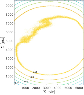
Figure 13. The typical vignetting pattern of a LAST telescope, as measured from a flat field image (after a 4 by 4 median filter). We assume that the pixel scale is uniform across the field of view. The vignetting was normalized to have a maximum of 1. Contour levels are shown in steps of 0.05.
Download figure:
Standard image High-resolution imageNormalizing the vignetting to have a peak value of 1, about 72% (93%) of the LAST image area has a vignetting >0.9 (>0.8).
7.2. Image Quality
Before applying tip-tilt corrections to the cameras, the measured FWHM, near the image center, ranges from 19 to 28. An example of the measured image quality in one of the telescopes/detectors before we applied tip-tilt correction is shown in Figure 14.

Figure 14. An example for the measured FWHM as a function of position on the detector. The FWHM was measured in bins of 800 by 800 pixels. In this example, the mean FWHM over the image is about 31.
Download figure:
Standard image High-resolution imageGiven the site median seeing of 14, the pixel scale of 125 pixel−1, and the theoretical delivered image quality these are reasonable performance results. Figure 15 shows several 15 s image cutouts around selected objects.

Figure 15. Small sections (out of the entire camera field of view) around selected objects. Exposure times are 15 s using a single telescope. Left to right, top to bottom are: NGC 253, M13, M57, the Veil, the Helix, and M42. NGC253 and M42 are presented in logarithmic scale.
Download figure:
Standard image High-resolution image7.3. Limiting Magnitude
Out of the three GAIA bands (Gaia Collaboration et al. 2016), the IMX455 sensitivity has the highest resemblance to the GAIA Bp band. Therefore, our calibration is done relative to this band. Here, we convert all the GAIA magnitudes to the AB magnitude system. This is done by adding 0.1136, 0.0155, and 0.3561 magnitude, to the G, Bp, and Rp GAIA Vega magnitudes, respectively. Figure 16 shows the S/N for detection versus the GAIA Bp magnitude for one representative (15 s) image taken at dark time near the zenith. Points with different colors represent sources with different Bp − Rp color (see legend). The colored lines show the logarithmic best-fit lines for sources in different color bins. The limiting magnitude for each image and coadd image is calculated by linear fitting the  as a function of the GAIA Bp magnitude and the Bp − Rp color. Next, the 5σ limiting magnitude is calculated by reading the value of the fitted function at S/N = 5 and Bp − Rp = 1.0 mag.

Figure 16. The Signal-to-Noise ratio (S/N) as a function of the Bp AB magnitude, for stars with different colors in a 15 s exposure (dots; color coding: see legend). The colored lines show the best fit  vs. Bp AB magnitude to stars in different color ranges. The limiting magnitude is estimated by reading the value of the fitted line at S/N = 5 and color equal 1.
Download figure:
Standard image High-resolution image
The typical, dark time, 5σ limiting magnitude in a 20 s exposure is about 19.6 (for V-band sky brightness of 21 mag arcsec−2). Using the coaddition of 20 × 20 s exposures the 5σ limiting magnitude, for Bp − Rp = 1.0 mag, is about 21.0. The system's limiting magnitude is color dependent, with a slope of +0.33 mag per Bp − Rp magnitudes. We estimate that building a LAST node in a dark-site location may improve its limiting magnitude by about 0.5 mag.
8. Maintance, Operations, and Lessons Learned
After the deployment of the telescopes, we encountered two major issues that are important to mention as a lesson for other efforts. The first problem was electromagnetic interference during communication (e.g., image transfer) with the cameras and, to a lesser extent, with the mounts. In most cases, the solutions to these problems are relatively straightforward to implement but hard to identify. The solutions include cable shielding, avoiding cables passing near electric systems, fixating the cable heads, and the addition of ferrites. The second major issue, which to some extent is still ongoing, is the enclosure reliability. This item likely requires a proper design.
The Neot-Smadar site was selected based on the speed of deployment considerations rather than site quality. A disadvantage of this site is due to dust that requires frequent cleaning of the computers, telescopes, and optics. Therefore, we spend about 1–2 hr per week on cleaning the observatory. Another minor maintenance issue is the low reliability of the electric focusers that we are using. For that reason, we have developed our own focuser that is currently being deployed.
9. Future Follow-up Facilities
Only about 10% of the transients currently found by sky surveys are being followed up spectroscopically (Kulkarni 2020). This is a big limiting factor that is likely to become even more problematic in the near future. Furthermore, for some applications, multi-band photometric observation is valuable for studying the objects of interest (e.g., for measuring bolometric light curves). However, LAST is designed as a discovery machine, and therefore it is normally not equipped with filters.
For these reasons, we designed two new follow-up facilities, one for photometric observations, and the second for spectroscopic follow-up. A major design goal of these new facilities is, again, cost-effectiveness.
The Pan-chromatic Array for Survey Telescopes (PAST) is a planned photometric telescope. The PAST design calls for four 14-inch f/11 telescopes on a single mount. Each telescope will be equipped with a dichroic filter and two cameras. The cameras will be equipped with broad-band filters (1500–2000 Å width). The eight filters on each mount will cover the 4000–8000 Å range with large overlaps, such that their linear combination will allow us to get photometry in 500 Å bands (see E. O. Ofek & B. Zackay 2023, in preparation). This will allow us, on one hand, to get deep, broad-band imaging, and on the other hand to obtain some spectral information. With the exception of the telescopes and dichroic filters, the PAST components are identical to those used in LAST.
The Multi-Aperture Spectroscopic Telescope (S. Ben-Ami et al. 2023, in preparation) will use a large number of small telescopes to collect the light from a target into a single spectrograph. Our goal is to be able to construct a telescope with a collecting area equivalent to a 2.7 m telescope, but for about 10% of the price of such a telescope.
10. Conclusions
We present the LAST project—A cost-effective high-grasp survey telescope for exploring the variable and transient sky. The first LAST node of 48, 28 cm telescopes, providing a total field of view of 355 deg2, is currently under construction. The first 12 telescopes saw their first light in early 2022 March, while an additional 20 telescopes were installed on 2023 March, and the rest are expected to be deployed by 2023 June. The development and construction time of LAST was relatively short—About three years from our first experimentation with the telescopes and some previous-generation camera and mounts we tested, to first light.
The LAST strategy of obtaining several images (the default is 20) of each field visit allows us, among other things, to identify minor planets, satellite glints, white dwarf transits, and flare stars (Ben-Ami et al. 2023). In turn, this provides a cleaner stream for transient detection. The LAST survey strategy will concentrate on a high cadence survey of the sky—this has the potential to open a new window into the fast transients and variability phase space (e.g., Drout et al. 2014; Ho et al. 2023; Ofek et al. 2021). Some initial science results from LAST are presented in Ofek et al. (2023).
An important aspect of the LAST design is its cost-effectiveness. In terms of volume of space per unit time per unit cost (i.e., grasp per unit cost), LAST is an order of magnitude improvement over most existing surveys. We believe that this point is important because it provides a path to construct affordable, very high grasp systems, around the globe. Such systems are needed in order to provide continuous monitoring of the sky and to probe the fast transients and variability phase space. Furthermore, with a large number of these systems, their collecting area will become competitive with existing large telescopes. We emphasize that this approach of multiple small telescopes can compete with large telescopes for seeing-limited observations, and likely also seeing-limited single-object spectroscopy (Section 9; Ofek & Ben-Ami 2020). However, large telescopes still have major advantages when equipped with diffraction-limited adaptive optics, K-band observations, multi-object spectroscopy, and additional unique instrumentation.
E.O.O. is grateful for the support of grants from the Willner Family Leadership Institute, André Deloro Institute, Paul and Tina Gardner, The Norman E Alexander Family M Foundation ULTRASAT Data Center Fund, Israel Science Foundation, Israeli Ministry of Science, Minerva, BSF, BSF-transformative, NSF-BSF, Israel Council for Higher Education (VATAT), Sagol Weizmann-MIT, Yeda-Sela, Weizmann-UK, the Rosa and Emilio Segre Research Award, Benozyio center, and the Helen-Kimmel center. A.F. and V.F.R. acknowledge support from the German Science Foundation DFG, via the Collaborative Research Center SFB1491: Cosmic Interacting Matters—from Source to Signal.
Footnotes
- 9
- 10
- 11
The 8-inch version, uses a different optical design with f/2 and its image quality is worse than the 11 and 14-inch telescopes.
- 12
Some tests are being performed with polarization filters.
- 13
In meridian observing strategy, this provides faster scanning.
- 14
We define this transition when the background variance is equal to the read-noise squared.
- 15
- 16
- 17