

Abstract
Several unexpected features have been observed in the microwave sky at large angular scales, both by WMAP and by Planck. Among those features is a lack of both variance and correlation on the largest angular scales, alignment of the lowest multipole moments with one another and with the motion and geometry of the solar system, a hemispherical power asymmetry or dipolar power modulation, a preference for odd parity modes and an unexpectedly large cold spot in the Southern hemisphere. The individual p-values of the significance of these features are in the per mille to per cent level, when compared to the expectations of the best-fit inflationary ΛCDM model. Some pairs of those features are demonstrably uncorrelated, increasing their combined statistical significance and indicating a significant detection of CMB features at angular scales larger than a few degrees on top of the standard model. Despite numerous detailed investigations, we still lack a clear understanding of these large-scale features, which seem to imply a violation of statistical isotropy and scale invariance of inflationary perturbations. In this contribution we present a critical analysis of our current understanding and discuss several ideas of how to make further progress.
Export citation and abstract BibTeX RIS
1. Introduction
Among the purposes of this contribution is to summarize the evidence for unexpected features of the microwave sky at large angular scales, as revealed by the observation of temperature anisotropies by the space missions Cosmic Background Explorer (COBE), Wilkinson Microwave Anisotropy Probe (WMAP) and Planck. Before doing so, let us put those discoveries into context with the study of other aspects of the cosmic microwave background (CMB) radiation.
Half a century ago, the discovery of the CMB revealed that most of the photons in the Universe belong to a highly isotropic thermal radiation at a temperature of ∼3 K [1]. Deviations from this isotropy were first found in the form of a temperature dipole at the level of ∼3 mK [2, 3]. This dipole has been interpreted as the effect of Doppler shift and aberration due to the proper motion of the solar system [4] with respect to a cosmological rest frame.
The observation of an isotropic CMB, together with the proper-motion hypothesis, provides strong support for the cosmological principle. This states that the Universe is statistically isotropic and homogeneous, and restricts our attention to the Friedmann–Lemaître class of cosmological models. The cosmological principle itself is a logical consequence of the observed isotropy and the Copernican principle, the statement that we are typical observers and thus observers in other galaxies should also see a nearly isotropic CMB.
The proper-motion hypothesis is supported by the COBE discovery of higher multipole moments [5]. These higher moments turned out to be two orders of magnitude below the dipole signal, at a rms temperature fluctuation of ∼30 μK at 10° angular resolution [6]. However, a direct test of the proper-motion hypothesis had to wait until Planck was able to resolve the Doppler shift and aberration of hot and cold spots at the smallest angular scales [7, 8]. It is important to note here that the observed dipole could also receive contributions from effects other than the solar system's proper motion. These could be as large as 40% without contradicting the Planck measurement at the highest multipole moments. Observations at non-CMB frequencies, e.g. in the radio or infrared, hint at significant structure dipoles or bulk flows, but are still inconclusive [9–19]. Here we dwell on this aspect as the CMB dipole is one of the most important calibrators in modern cosmology. It defines what we call the CMB frame and many cosmological observations and tests refer to it.
The existence of structures like galaxies, voids and clusters imply that the CMB cannot be perfectly isotropic. The COBE discovery [5] revealed the long-expected temperature anisotropies and confirmed that they are consistent with an almost scale-invariant power spectrum of temperature fluctuations. Scale invariance of the temperature anisotropies means that the band power spectrum  is a constant for small multipole number ℓ. Here
  denotes the expected variance in the amplitude of any spherical harmonic component of the temperature fluctuations with total angular-momentum5
ℓ.
denotes the expected variance in the amplitude of any spherical harmonic component of the temperature fluctuations with total angular-momentum5
ℓ.
During the last two decades, ground-based, balloon-borne and satellite CMB experiments led to an improved understanding of those temperature anisotropies. The WMAP and Planck space missions played a special role, obtaining full-sky measurements that enabled us to investigate a large range of angular scales, from the dipole  to
to  , more than three decades in ℓ. The band power spectrum as published by Planck is shown in figure 1.

Figure 1. Angular band power (top) and residual angular band power (bottom) of the cosmic microwave temperature anisotropies as presented in the Planck 2015 release [20] reproduced with permission © ESO. The error bars show the sum of measurement error and cosmic variance, the latter being the dominant source of uncertainty at large angular scales.
Download figure:
Standard image High-resolution imageThese temperature fluctuations are believed to have been generated from quantum fluctuations in the very early Universe [21] by a (nearly) scale-invariant mechanism. The most prominent context is cosmological inflation [22, 23]. If inflation lasts long enough, the spatial geometry of the Universe is generally predicted to be indistinguishable from Euclidean, and the topology of the observable Universe is expected to be trivial (simply connected). Even more importantly, inflation predicts that the CMB temperature fluctuations should be: (i) statistically isotropic, (ii) Gaussian, and (iii) almost scale invariant. It also predicts: (iv) phase coherence of the fluctuations; (v) for the simplest models, a dominance of the so-called adiabatic mode (strictly speaking it is not only adiabatic but also isentropic); and (vi) the non-existence of rotational modes at large scales. Finally, depending on the energy scale of cosmological inflation, there might be (vii) a detectable stochastic background of gravitational waves [24] that also obeys properties (i)–(iii).
In the process of extracting cosmological parameters from the CMB and other observations, properties (i)–(vi) are assumed to hold true and a stochastic gravitational wave background is neglected. This leads to the minimal inflationary Λ cold dark matter (ΛCDM) model [25].
Analysis of the CMB allows us not only to fit all free parameters of this model, but also to test its underlying assumptions. However, the more fundamental the assumption, the harder it appears to test. The existence of the peaks and dips shown in figure 1 are due to the phase coherence, property (iv). The almost-scale-invariance (iii) is visible in the smallness of the deviations from the best-fit model, although a model-independent reconstruction of the primordial power spectrum leaves room for deviations at the largest observed scales [26]. More detailed analysis also reveals that there is a strong upper limit of at most 4% of non-adiabatic modes (v) [26], while rotational modes would have produced a large B-polarization signal that is not observed. The predicted flatness and the expected trivial topology are consistent with all observations [27, 28].
It thus remains to test Gaussianity and statistical isotropy. A lot of effort has been put into searches for non-Gaussianity and they are described in great detail elsewhere. The brief summary is that there is no evidence for it so far [29]. In the following we focus our attention on statistical isotropy, and touch on the issue of scale invariance.
All mentioned predictions should hold at all observable scales. However, testing these primordial properties of the Universe directly is complicated by physics related to the evolution of the Universe after the end of cosmological inflation. In order to understand which phenomena can be most cleanly probed at which scales it is instructive to look at the comoving size corresponding to a particular angular scale as a function of redshift, see figure 2.

Figure 2. The comoving length of an arc on the sky with opening angle of 180°, 60°, 20° and 1° is compared to the comoving Hubble distance. Angular scales larger than  ° can only be affected by primordial physics or physics at redshift
  , corresponding to the present (the reionized, the transparent) Universe. The shaded region indicates scales and redshifts on which structure formation is expected to generate density contrasts of order 0.1 or larger.
Download figure:
Standard image High-resolution imageAt the time of the formation of the first atoms, scales that today subtend more than about a degree (and that therefore affect  ) were not much affected by details of photon decoupling. Thereafter, the Universe was filled with a mix of H and He gas, until it was reionized at a redshift of about 10. Angular scales larger than about 20° (or
  ) are also not much affected by the details of reionization. Finally, angular scales larger than
  (or
(or  ) enter the Hubble scale at a redshift of one and thus are either of primordial or local origin. Here by local we mean from within our Hubble patch of the Universe. Thus it is a good idea to start with a test of statistical isotropy at the largest angular scales, as whatever we find must be either primordial or a local effect due to either foreground or local cosmic structure.
In this contribution we intend to give a summary of the evidence for the existence of features of the microwave sky that apparently violate statistical isotropy on the largest angular scales (section 2). Since this seems to happen only at the largest angular scales, it also amounts to a violation of scale invariance. We also discuss several ideas that have been put forward to explain those features, though we do not intend to give an exhaustive review. Apart from the suggestion that all of them are statistical flukes (the probability for which to happen is tiny, unless compensated for by huge look-elsewhere penalties) these ideas can be classified into foreground effects (section 3) and cosmological effects (section 4). In section 5 we highlight several possible tests of those ideas. The study of polarization at large angular scales and more detailed all-sky study of non-CMB wavebands seems to be particularly promising.
2. A summary of the evidence
Some of the unexpected features in the CMB temperature anisotropies have been identified in angular space,  , where
  is a unit vector describing a position on the sky, and some in harmonic space

where  denote spherical harmonic functions. Mathematically, all of the information in a full-sky map,
  , is contained in the
  . However, as one often finds in transforming data, the different representations can reveal complementary features. Furthermore, many of the usual relationships between angular-space and harmonic quantities are complicated by the presence of the galactic foreground, which forces us to mask, weight and clean the observed maps. Thus it is advisable and fruitful to study both sides of the spherical-harmonic coin.
For a statistically isotropic sky, the one-point expectation values are  and
and  , both quantities with an arbitrarily large cosmic variance, thus T0 cannot be predicted. It is a free parameter of the ΛCDM model and must be measured, which was first done by Penzias and Wilson [1] and most accurately to date by COBE [30, 31]. We also employ the usual hypothesis of the observed dipole being purely due to our proper-motion and thus only consider harmonic modes with
  in the discussion below.
Harmonic techniques seem to be much better suited than angular-space methods for extracting ΛCDM model parameters. One reason is that for statistically isotropic skies the harmonic coefficients are orthogonal in a statistical sense (i.e. uncorrelated)

For Gaussian harmonic coefficients, all information is encoded in the angular power spectrum  .
.
In angular space, the two-point correlation function of a statistically isotropic sky

does not have the property that  is independent from
  for
for  . Thus it seems to be easier to draw inferences from the angular band power spectrum than from the angular two-point correlation function. On the other hand, if a feature is attached to a certain region of the sky, or otherwise violates statistical isotropy, it may be much harder to spot it in the harmonic analysis than in angular-space.
The issue of cosmic variance is important for the analysis of the largest cosmological scales. For statistically isotropic and Gaussian skies, the estimation of the angular power spectrum  is limited by the fact that we can only observe one particular realization of the horizon-size region of the Universe. For full sky observations the estimator

is unbiased ( ) and minimizes variance6

The expression in equation (5) is the sample variance which, in cosmology, is usually referred to as the cosmic variance: this is an irreducible lower bound on the error in the measurements of the angular power spectrum coming from the fact that we observe fluctuations in only one Universe. The cosmic variance of the angular power spectrum also leads to a non-zero cosmic variance of estimates of the two-point correlation  . The cosmic variance further increases when foreground dominated regions are masked in the data analysis. All results quoted below take these aspects fully into account.
A summary of the most important findings in angular and harmonic space is provided in table 1.
Table 1.
P-values in per cent of various unexpected features. In this table we define the sense of p-values such that a small value means that it is unexpected. In some cases this is different from the sense used by the Planck collaboration in their analysis. The Planck analysis relies on just 1000 Monte Carlo simulations of the instrument and pipeline and thus p-values below  cannot be resolved. Other groups have used larger numbers of simulations, but those simulations do not include instrumental and algorithmic effects of the Planck analysis. LEE stands for look elsewhere effect.
| Feature | p-value | Data | Reference |
|---|---|---|---|
| In angular space | |||
low variance ( ) ) |
≤0.5% | Planck 15 | Table 12 [8] |
2-pt correlation 
|
≤3.2% | Planck 15 | Table 14 [8] |
2-pt correlation 
|
≤0.5% | Planck 15 | Table 13 [8] |
2-pt correlation 
|
≤0.3% | Planck 13 and | |
| WMAP 9 yr | Table 2 [34] | ||
2-pt correlation  (larger masks) (larger masks) |
≤0.1% | Planck 13 | Table 2 [34] |
| ≤0.1% | WMAP 9 yr | [34, 35] | |
| Hemispherical variance asymmetry | ≤0.1% | Planck 15 | Table 20 [8] |
| Cold spot | ≤1.0% | Planck 15 | Table 19 [8] |
| In harmonic space | |||
| Quadrupole–octopole alignment | ≤0.5% | Planck 13 | Table 7 [36] |
 alignment alignment |
≤0.2% | Planck 13 | Table 7 [36] |
Odd parity preference 
|
≤0.3% | Planck 15 | Figure 20 [8] |
Odd parity preference  (LEE) (LEE) |
≤2% | Planck 15 | Text [8] |
Dipolar modulation for 
|
≤1% | Planck 15 | Text [8] |
2.1. Low variance and lack of correlation
Historically, the first surprise, already within the COBE data, was the smallness of the quadrupole moment. When WMAP released its data [32], it confirmed C2 to be low, however it was also shown that cosmic variance allows for such a small value [33].
Another rediscovery in the first release of WMAP [32] was that the angular two-point correlation function at angular scales  ° is unexpectedly close to zero, where a non-zero correlation signal was to be expected. This feature had already been observed by COBE [37], but was ignored by most of the community before its rediscovery by WMAP. The two-point correlation function as observed with Planck [8] is shown in figure 3.

Figure 3. Angular two-point correlation function as observed by Planck [8] reproduced with permission © ESO. The full black line and the shaded regions are the expectation from 1000 SMICA simulations based on the ΛCDM model and the 68% and 95% confidence regions. The plot also shows four colored lines that fall on top of each other and represent the result of the Planck analysis of the Commander, SEVEM, NILC and SMICA maps at resolution  . While the measured two-point correlation is never outside the 95% confidence region, the surprising feature is that we observe essentially no correlations at
  and a significant lack of correlations at
  .
.
Download figure:
Standard image High-resolution imageThe WMAP team suggested a very simple statistic [38] to characterize the vanishing correlation function

with  . This measures the deviation from zero at
  . Detailed further investigations of the lack of angular correlation have been presented in [34, 35, 39–41]. Depending on the details of the analysis, p-values consistently below
  have been obtained, some even below
  . An important question is the size of the mask used in the analysis. It has been shown in [40] that most of the large-angle correlations in reconstructed sky maps are between pairs of points at least one of which is in the part of the sky that is most contaminated by the Galaxy. This is in line with the findings of [35], where it was shown that more conservative masking makes the lack of correlation even more significant. This by itself already signifies a violation of isotropy.
Undoubtedly,  is an ad hoc and a posteriori statistic, but it captures naturally the observed feature originally noted in COBE. Several a posteriori 'improvements' have been suggested [8, 42]. For example, in order to avoid the argument that
  has been fixed after the fact one might let μ vary. But now the look elsewhere effect must be taken into account. The Planck team implemented such an analysis which (in our convention) returns global p-values of the order of 2%. However, this global Sμ statistic addresses a different question, namely how likely is it that there is a lack of correlation for an arbitrary μ. Thus we cannot argue that this statistic is better than
  , all we can say is that it is different.
Another critique was that the  statistic does not account for correlations among
  at different θ [42]. Such a correlation is indeed expected in the ΛCDM model, but if we would use that fact, we would be injecting a model assumption into the data analysis. Thus the recent Planck analysis [8] tests the
  statistics, which compares the data to the ΛCDM expectation, and a
  statistics, which tests for the non-vanishing of
  assuming the ΛCDM covariance. The p-values for both tests are around 3% and 2%. Let us add that the recent Planck analysis is based on a resolution of
  and relies on a mask that includes 67% of the sky for cosmological analysis. It was shown recently in [43] that enlarging that mask gives rise to significantly smaller p-values and increased evidence of a lack of correlation.
It has further been suggested [44] that the two-point correlation function calculated directly on a cut sky is a suboptimal estimator of the full-sky two-point correlation function, and that better estimators lead to less statistical significance for the observed anomalies. This result has been extended [45] to all anisotropic Gaussian theories with vanishing mean. We however think that the issue of the optimality of the full-sky estimator is irrelevant, since it is the cut-sky two-point correlation function which is observed to be strikingly anomalous, and which begs an explanation [34].
Another very simple statistic is to calculate variance, skewness and kurtosis of the unmasked pixels. In this test the Planck team found evidence for low pixel variance for low-resolution maps ( ), while skewness and kurtosis behave as expected [8, 46]. This feature seems to be consistent with a low quadrupole, a lack of power at large angular scales (for
  , see figure 1) and the discussed lack of angular correlation. The latter cannot be explained by a lack of quadrupole power alone. All modes below
  contribute to the observed lack of angular correlation [40]—not by having low amplitudes, but by combining to cancel one another and the contributions of still higher ℓ. This is indicative of correlations among
  not predicted by the ΛCDM model and a violation of both statistical isotropy and scale invariance.
It has been noted [34] that what is reported as the two-point angular correlation function  is actually the dipole (and monopole) subtracted two-point angular correlation function. A cosmological dipole of the size expected in the best-fit ΛCDM model would completely dominate
  . In order not to raise
  significantly above its dipole-subtracted value, one must have
  , compared to the value of approximately
  that standard CMB codes return. Of course even the latter is orders of magnitude smaller than the dipole that we measure, which we interpret to be entirely due to the observer's motion with respect to the rest frame of the CMB (and hence excluded from
  ). There is disagreement over whether the intrinsic CMB dipole is physical or observable. It is certainly likely to be difficult to measure the dipole to the necessary parts in 104, to begin distinguishing the intrinsic dipole, in any, from the
  mK Doppler dipole.
2.2. Alignments of low multipole moments
In the standard ΛCDM model the temperature (and other) anisotropies have random phases. In harmonic space this means that the orientations and shapes of the multipole moments are uncorrelated. This was first explored in the first year WMAP data release using the angular momentum dispersion [47] where it was discovered that the octopole ( ) is somewhat planar (dominated by
  for an appropriate choice of coordinate frame orientation) with a p-value of about 5%. (A quadrupole is always planar.) More importantly, the normal to this plane (the axis around which the angular momentum dispersion is maximized) was found to be surprisingly well aligned with the normal to the quadrupole plane at a p-value of about
  .
.
Subsequently these ideas have been studied in more detail using other measures of planarity and alignment [36, 41, 48–50]. A convenient tool for such a study are the Maxwell multipole vectors [51]. They provide an alternative to the spherical harmonics as a means to represent angular momentum ℓ objects in a manifestly symmetric, rotationally invariant manner. Roughly speaking they represent the multipole moments by products of unit vectors. A dipole is a vector. A quadrupole can be constructed from the product of two dipoles (two vectors), an octopole from three dipoles (three vectors), and so on for arbitrary multipole moment ℓ. Of course two dipoles produce both quadrupole and monopole moments so only particular combinations of the products of dipoles will produce a pure quadrupole. Mathematically they are represented by the trace-free product of the two dipoles. In the end this means an angular moment ℓ object can be represented by ℓ unit vectors and an overall amplitude (put together these contain the requisite  degrees of freedom).
Given the multipole vectors,  for i = 1 to ℓ, questions about alignments can now be addressed. It has been found convenient to directly study not the multipole vectors but instead their oriented areas [51]

defined for each pair of multipole vectors at a fixed ℓ. Notice that these are not unit vectors, their magnitudes are the area of the parallelogram created by the two vectors. These oriented-area vectors can then be compared among the multipoles or to fixed directions. The multipole vectors for the quadrupole and octopole along with the oriented area vectors, their maximal angular momentum dispersion directions  , and some special directions are shown in figure 4.

Figure 4. The combined quadrupole–octopole map from the Planck 2013 release [36]. The multipole vectors (v) of the quadrupole (red) and for the octopole (black), as well as their corresponding area vectors (a) are shown. The effect of the correction for the kinetic quadrupole is shown as well, but just for the angular momentum vector  , which moves towards the corresponding octopole angular momentum vector after correction for the understood kinetic effects.
Download figure:
Standard image High-resolution imageNumerous statistics can be defined to quantify alignment; here we only consider one. Since the multipole vectors really only define axes (both  are multipole vectors) we define the S statistic as

Here  represents a fixed direction on the sky and
  represents one of the oriented-area vectors. The sum is over some set of oriented-area vectors. Although this can be used with any set of multipole vectors and/or directions here we focus on two cases. First, the quadrupole–octopole alignment where we use
  (the oriented area vector for the quadrupole) as the fixed direction called
  above and the
  are the three oriented-area vectors for the octopole,
  . Second, the joint alignment of the quadrupole and octopole with special directions such as the normals to the ecliptic and to the Galactic planes or the direction of our motion with respect to the CMB (the dipole direction). In this latter case the
  refer to the quadrupole oriented-area vector and the three such vectors from the octopole (so that n = 4).
The most recent analysis of the latest WMAP and the Planck 2013 data releases [36] finds the quadrupole and octopole anomalously aligned with one another, with p-values ranging from about  –2% depending on the exact map employed. It is further found that the quadrupole and octopole are jointly perpendicular to the ecliptic plane (i.e. their area vectors are nearly orthogonal to the normal to the ecliptic) with a p-value of 2%–4% and to the Galactic pole with a p-value of 0.8%–1.6%. Even more strikingly they are aligned with the dipole direction with a p-value of 0.09%–0.37% .
A number of issues must be considered when interpreting the p-values given above. Arguably, it is surprising not only that these alignments are observed at all but that they have persisted in the data from the original WMAP data release to the present. To study the alignments (phase structure of the temperature fluctuations) full-sky maps are required. Thus the results of [36] are based on the cleaned maps produced by WMAP (the ILC maps) and from different cleaning methods employed by Planck (NILC, SEVEM, and SMICA). The exact phase structure of the maps is sensitive to many effects including the details of the cleaning algorithms, systematics effects in interpreting the data (such as the beam profile) which have been improved through the years, and the different observation strategies employed by WMAP and Planck. Despite the many effects that could have masked the alignments, they persist in the data and remain to be understood.
Our motion with respect to the rest frame of the CMB contributes not only to the dipole, as mentioned above, but also to all other higher multipole moments. The effect of our motion in mixing two multipole moments ℓ and  is suppressed by
  with
with  . The monopole therefore contaminates mostly the dipole, and has little effect on the power spectrum for
  . Other multipoles mix only slightly, since they have comparable
  to begin with. (Actually, the mixing effect is
  , so there is significant mixing at
  , but we will not concern ourselves here with such high ℓ.) However, the so called kinetic quadrupole does affect the phase structure for
  [48], as seen in figure 4. The direction of the quadrupole oriented-area vector, labeled by Qa and
  in the figure, shifts by about 5° from the 'no DQ' value (diamond) to the corrected value (square) when the kinetic quadrupole moment due to our motion is removed from the full-sky temperature map prior to analysis. The amplitude of the kinetic quadrupole is frequency dependent and the cleaned, full-sky maps are constructed from linear combinations of observations in many frequency bands making the exact kinetic quadrupole calculation difficult to calculate. This is exacerbated by calibration techniques which sometimes subtract some of the frequency dependent kinetic quadrupole contribution. The Planck 2013 data release provided estimates for the required correction factor [46] beyond the simple estimate used in the results quoted above. Interestingly when these corrections are applied the alignment becomes even more anomalous. For example, the p-value for the alignment with the dipole direction drops to between
  and
and  [36], or even less [52]. The angular momentum quadrupole–octopole alignment and the increase of the alignment due to the kinetic effect has also been confirmed for the Planck 2015 data set [53].
In summary, the octopole is unexpectedly planar; the quadrupole and octopole planes are unexpectedly aligned with each other, and unexpectedly perpendicular to the ecliptic and aligned with the CMB dipole. These alignments have been robust in all full-sky data sets since WMAP's first release, and are found to be exacerbated by proper removal of the kinetic quadrupole. No systematics and no foregrounds have been identified to explain these apparent violations of statistic isotropy.
2.3. Hemispherical asymmetry
Evidence for hemispherical power asymmetry first emerged in the analysis of WMAP first-year data [54, 55]. It was found that the power in disks on the sky of radius ∼10°–20°, evaluated in several multipole bins, is larger in one hemisphere on the sky than the other; see the left panel of figure 5. The plane that maximizes the asymmetry is approximately the ecliptic, though it depends somewhat on the multipole range; the variation of the normal to this plane with multipole range is shown in the right panel of figure 5. Figure 4 shows that the combined quadrupole and octopole moment already contribute to such a power asymmetry.

Figure 5. Hemispherical power asymmetry. Left panel: original evidence, adopted from [54]. The three jagged lines show the binned angular power spectrum calculated over the whole unmasked sky (dashed), northern hemisphere (solid line, with crosses), and southern hemisphere (dotted line, with circles). North and south were defined with respect to the best-fit axis for WMAP1 data, and were close (but not identical) to the north and south ecliptic. The histogram and the two gray areas around it denote the mean and the 68% and 95% confidence regions from Gaussian random simulations. Right panel: best-fit directions from the dipolar modulation model, applied to Planck 2015 SMICA map, evaluated in multipole bins centered at 50–1450 [8]. Directions corresponding to the North ecliptic pole (NEP) and South ecliptic pole (SEP), the CMB dipole, and the best-fit WMAP9 modulation direction are also shown. The 'low-l' direction refers to constraining  , while the blue and brown rings show analysis in the two multipole ranges
 ![${\ell }\in [2,300]$](https://content.cld.iop.org/journals/0264-9381/33/18/184001/revision1/cqgaa345bieqn95.gif) and
and ![${\ell }\in [750,1500]$](https://content.cld.iop.org/journals/0264-9381/33/18/184001/revision1/cqgaa345bieqn96.gif) , respectively.
, respectively.
Download figure:
Standard image High-resolution imageThe study of hemispherical asymmetry was extended to later years of WMAP [56–58] as well as Planck [8, 46, 58] by analyses that modeled the asymmetry as a dipolar modulation [59, 60]

where  and
and  are the modulated and unmodulated temperature fields, respectively,
  is an arbitrary direction on the sky, and A and
  are the dipolar modulation amplitude and direction. This parameterization enables a straightforward Bayesian statistical analysis. The earlier analyses have found statistically significant evidence for
  , and direction
  roughly in the ecliptic pole direction. The result from the Planck 2015 release, using the Commander map, is
  with
with  pointing in the direction
  [8].
[8].
It has been pointed out in [61, 62] that this modulation is not scale invariant, i.e. the amplitude A is a function of multipole range. The modulation's direction is remarkably consistent as a function of the multipole range used, and between WMAP and Planck, as the right panel of figure 5 shows. Planck also finds that the modulation, as measured by the coupling of adjacent multipoles, has most signal at relatively low multipoles, ![${\ell }\in [2,67]$](https://content.cld.iop.org/journals/0264-9381/33/18/184001/revision1/cqgaa345bieqn106.gif) where it has a p-value of 1%. In figure 6 the dipolar directions found in Planck 2015 data [8] by means of a bipolar spherical harmonics analysis [63, 64] are shown. At low multipoles the same direction in the Southern ecliptic hemisphere is identified (left panel), while at much higher multipoles the Doppler boost and aberration dipolar modulation (due to the proper motion of the solar system) is picked up (right panel).
where it has a p-value of 1%. In figure 6 the dipolar directions found in Planck 2015 data [8] by means of a bipolar spherical harmonics analysis [63, 64] are shown. At low multipoles the same direction in the Southern ecliptic hemisphere is identified (left panel), while at much higher multipoles the Doppler boost and aberration dipolar modulation (due to the proper motion of the solar system) is picked up (right panel).

Figure 6. Results of bipolar spherical harmonics analysis [8] reproduced with permission © ESO. Left: dipolar modulation, only darkest blue spot is statistically significant ( to 64). Right: Doppler modulation at high ℓ.
Download figure:
Standard image High-resolution imageA different way to measure the hemispherical asymmetry is to consider variance calculated on hemispheres. References [58, 65] found that the northern hemisphere in WMAP 9 year and Planck 2013 maps has an extremely low (significant at 3– ) variance evaluated on scales 4°–14° relative to what is expected in the ΛCDM model. Planck [8] found that the result holds at an even wider range of scales once the lowest harmonics (
 ) are filtered out from the map. Moreover, configurations of the three and four-point correlation function, evaluated at a resolution of7
Nside = 64 (that is, down to
) are filtered out from the map. Moreover, configurations of the three and four-point correlation function, evaluated at a resolution of7
Nside = 64 (that is, down to  on the sky) also exhibit the hemispherical asymmetry. Finally, evidence for hemispherical asymmetry in WMAP data was also found by measuring power in disks of fixed size on the sky [67].
The fact that the axis that maximizes the asymmetry is close to the ecliptic pole motivates both systematic and cosmological proposals for the hemispherical asymmetry. Nevertheless, there have been no convincing proposals to date about why one ecliptic hemisphere should have less power than the other.
2.4. Parity asymmetry
It is interesting to ask whether the CMB sky is, on average, symmetric with respect to reflections around the origin,  . The standard theory does not predict any particular behavior with respect to this point-parity symmetry. Because
  , even (odd) multipoles ℓ have an even (odd) symmetry.
Tests of parity of the CMB have first been discussed in [68], who studied both the aforementioned point-parity symmetry, and the mirror parity ( , with
  being the axis normal to the mirror plane). The point-parity symmetry analysis of WMAP maps was extended by [69–71] who studied the even and odd parity maps

Using a suitably defined power spectrum statistic—the ratio of the sum over multipoles of  for the even map to that for the odd map—they found a
  evidence for the violation of parity in WMAP7 data in the multipole range
  . The analysis was finally extended to Planck by [8, 46], who confirmed the results from [69] based on WMAP, but also found that the significance depends on the maximum multipole chosen, and peaks for
  , but is lower for other values of the maximum multipole used in the analysis; see figure 7. The corresponding p-values of the Planck 2015 analysis, also including the 'look elsewhere' effect with respect to the choice of
  , are reported in table 1. Planck also studied the mirror symmetry, finding less anomalous results than those for the point-parity symmetry [8].

Figure 7. Parity asymmetry in the Planck 2015 data [8] reproduced with permission © ESO. Shown is the p-value significance, based on a power-spectrum statistic sensitive to parity for the four foreground cleaned Planck maps (Commander, NILC, SEVEM and SMICA) as a function of the maximum multipole used in the analysis.
Download figure:
Standard image High-resolution imageIn [72] it was shown for WMAP 7 years data that the directions of maximal (minimal) parity asymmetry for multipole moments up to  , and excluding the m = 0 modes from the analysis, seem to be normal (parallel) to the direction singled out by the CMB dipole. The direction that maximizes this parity asymmetry is also close to the direction of hemispherical asymmetry when including the lowest multipole moments. Thus parity asymmetry and hemispherical asymmetry might be linked to each other.
Whether the observed parity asymmetry is a fluke, an independent anomaly, or a byproduct of another anomaly, is not clear at this time. The parity asymmetry appears to be correlated with the missing power at large angular scales, as the wiggles in the lowest multipoles, seen clearly in the top panel of figure 7, combine to nearly perfectly cancel the angular two-point correlation function above 60° [40].
2.5. Special regions: the cold spot
Evidence for an unusually cold spot in WMAP 1st year data was first presented in [73]. The spot, shown in figure 8, is centered on angular coordinates  , has a radius of approximately five degrees, is roughly circular [74], and the evidence for its existence is frequency independent [73]. The cold spot was originally detected using spherical Mexican hat wavelets, which are well suited for searching for compact features on the sky; tests in [73] detected a deviation from the Gaussian expectation in the kurtosis of the wavelet coefficients at the wavelet scale of
  . Taking into account the 'look elsewhere' effect, that is the fact that not all statistics attempted with the wavelets returned an anomalous result, [75] estimated the statistical level of anomaly of the cold spot to be
  .
.

Figure 8. Cold spot in WMAP 7th year temperature maps. Left panel shows the map with the circle. Middle panel is the more detailed picture of the spot, while the right panel is the wavelet-filtered version of the middle panel (wavelet size  ). The small spots in the right panel are regions of known point sources that have been masked). All figures are adopted from the review in [86].
Download figure:
Standard image High-resolution imageThese original detections were followed up, confirmed, and further investigated using not only Mexican hat wavelets [76, 77], but also steerable [78] and directional [79] wavelets, needlets [80, 81], scaling indices [82], and other estimators [83]. The detection of the cold spot has also been challenged by [84] on grounds that alternative statistics—say, over/under density at disks of varying radius—does not lead to a statistically significant detection once look-elsewhere effects are taken into account. While the lingering worries about a posteriori nature of this particular anomaly make its significance difficult to quantify, the basic existence of the cold spot seems to be confirmed by most analyses. For comprehensive overviews of the cold spot, see [85, 86].
The intermediate size of the cold spot, as well as its frequency independence, argue against simplest systematic and foreground explanations. The size of the cold spot ( ) makes it too large to be a point source, yet typically too small to be a diffuse foreground, especially since it is found in a relatively foreground-clean part of the sky. And while the Sunyaev–Zeldovich effect—inverse Compton scattering of the CMB photons off hot electrons in Galaxy clusters—could in principle lead to the desired amplitude and spatial extent of the signal, the SZ effect has a very pronounced frequency dependence that is completely incompatible with the observed frequency independence of the cold spot signal [74].
Recent developments in the search for links between CMB cold spots and underdensities in the Galaxy distribution, discussed further in section 5.2, are of particular interest. While it is in principle possible that an underdensity in the Galaxy and dark matter distribution be responsible for the CMB cold spot [87], such a void would have to be huge, and therefore fantastically unlikely in the standard ΛCDM cosmology, making it much less probable than the CMB cold spot itself. One could nevertheless search for the link between the CMB cold/hot spots and Galaxy under/overdensities. The most general way to search for such a link is to cross-correlate the CMB temperature with the Galaxy overdensity over the whole observed sky (for each), but such tests have not shown evidence for departures from the ΛCDM prediction (e.g. [88]). However, it is possible that the cross-correlation performed more selectively—e.g. looking for CMB overdensity behind clusters of galaxies or voids [89, 90] or, taken to extreme, behind the cold spot alone [91, 92]—would indeed show departures from ΛCDM predictions. Such tests performed to date have shown tantalizing, though as yet not definitive, evidence for a large underdensity in the distribution of galaxies in the same direction as the cold spot; this is further discussed in section 4.2.
If the cold spot is indeed taken as a sign of departure from the ΛCDM model's predictions, it may be possible to explain it using novel theory. In the context of cosmological inflation, it has been suggested that a local perturbation in a spectator field could be transferred to a localized curvature perturbation during reheating and generate a local over- or underdensity like the cold spot [93, 94]. A theoretical explanation has a challenge of generating a localized feature of a rather small size ( ) in a non-special direction on the sky. In this regard, Bianchi cosmological models that are homogeneous but not isotropic are well suited and have been proposed as the explanation of the cold spot [95]. Another possibility that has been discussed is the presence of cosmic textures [96, 97], defects whose profile parameters can be chosen to explain the cold spot. While the texture explanation is favored by the Bayesian analysis [96] and appears viable in principle, it seems difficult to make further progress without independent predictions made by the texture model and their confirmation with future data.
2.6. Special regions: loop A
In the context of the study of a possible foreground from radio loops (see section 3), a huge loop, named loop A, has been identified in the vicinity of the cold spot [53]. Masking this particular region of the sky reduces the significance of the parity asymmetry, and the significance of dipolar modulation, and this region might largely be responsible for the observed quadrupole–octopole pattern. However, a corresponding foreground has not yet been identified.
2.7. Statistical independence of CMB anomalies
Although most of the described features or anomalies show p-values in the per cent or per mille level, none of them individually reaches the  detection level that is adopted in particle physics. Whether such a strong criterion is actually necessary or not might be debated. However, it is extremely hard to believe that our realization of ΛCDM just happens to have all of these features by chance, unless they have a common origin. It might be that some of the features result in other features, e.g. a low quadrupole clearly contributes to the low variance and vice versa. Thus in order to better characterize the CMB anomalies it would be useful to reduce them to a few 'atoms', i.e. a set of mutually independent features when analyzed in the context to the inflationary ΛCDM model. This study is an ongoing program, and is computationally expensive, as it requires large sets of Monte Carlo studies (many more than produced for the Planck full focal plane simulations [98]).
Here we propose such a set of 'atoms' that are independent of each other in the context of the ΛCDM model. At the present time we think that there are at least three such 'atoms': lack of angular correlation at large angles, alignments of the lowest multipole moments, and hemispherical power asymmetry.
The first 'atom', the lack of correlation, can also cause a low quadrupole and low variance, while for example a low quadrupole alone, cannot cause a lack of correlation. Detailed studies of constrained simulations have shown that a lack of correlation does not increase the chances to find alignments, and aligned multipoles do not increase the probability to find a lack of correlation [99, 100]. It has also been investigated if an intrinsic alignment of quadrupole and octopole correlates with the extrinsic alignment with some other directions, such as the dipole, ecliptic or galactic planes. These tests have been inconclusive [36]. We thus conclude that the mutual alignment of the lowest multipole moments is the second anomaly 'atom'.
The observed dipolar modulation seems to be also independent of the alignments between multipole moments. We propose that to be the third 'atom'. In [101] the p-values for various alignment measures were compared to the predictions of ΛCDM and a dipolar modulated model [59]. They showed that in both cases the alignment p-values are of the order of  . To our knowledge an explicit test in which the lack of angular correlation is correlated with dipolar modulation has never been done. The Planck team has also shown that a high-pass filter, which suppresses the multipole moments at
  actually increases the significance of the hemispherical variance asymmetry [8]. This shows that the quadrupole–octopole pattern alone is not responsible for most of the hemispherical asymmetry signal; moreover, the maximal asymmetric directions for
  and
and  do not agree, which is yet another indication that we face at least three independent 'anomaly atoms'.
One of those 'atoms' could certainly be an unlikely statistical fluke, however, it is quite unlikely that two of them, or even all three of them are statistical flukes (the corresponding p-values would be at most  ). This means that these anomalies could rule out the inflationary ΛCDM model and herald a new model in which those anomalies become a feature. The open question is, which of those features hold the key to decipher the underlying physical mechanism(s).
3. Foregrounds
If these anomalous CMB features are related to local physics, it might not be surprising that they appear to be a rare fluke. The reason is simple—our environment is one particular example of an environment for a CMB mission and every particular realization is somewhat special. In this section we review some of the local physical effects that have been suggested as explanations for CMB anomalies. We ignore speculations on instrumental effects, as it seems to us that the consistency of WMAP and Planck 2015 results [20] makes such an explanation quite unlikely.
3.1. Solar system
The closest foreground to a CMB space mission is the solar system itself. An obvious (subdominant) source of microwave radiation is the dust grains, and their emission might contribute to or modify the observed CMB anomalies [103–105]. The zodiacal cloud has been studied in detail for the Planck 2013 release [106] and the Planck team in its 2015 analysis subtracted a fit to the Kelsall model for the zodiacal cloud before map making [20]. The Kelsall model [107] attempts to capture the solar system dust emission in the infrared and microwaves and is based on the analysis of COBE DIRBE observations.
When comparing the Kelsall model with two meteoroid engineering models (used by space agencies to reduce the hazard to launch a spacecraft into a shower of meteoroids), it has been found that those engineering models [108, 109], depending on the chemical composition of the dust grains, predict a much brighter zodiacal cloud at microwave frequencies [102]. The Divine model of the interplanetary meteoroid environment [108] predicts meteoroid fluxes on spacecraft anywhere in the solar system from 0.05 to 40 AU from the Sun. This model uses data from micro-crater counts in lunar rocks from Apollo, meteor radar, and in situ measurements from Helios, Pioneer 10 and 11, Galileo and Ulysses. However, it does not make use of the infrared observations of COBE DIRBE. The Interplanetary Meteoroid Engineering Model (IMEM) [109] and the Divine model use the distributions in orbital elements and mass rather than the spatial density functions of the Kelsall model, ensuring that the dust densities and fluxes are predicted in accord with Keplerian dynamics of the constituent particles in heliocentric orbits. IMEM is constrained by the micro-crater size statistics collected from the lunar rocks, COBE DIRBE observations of the infrared emission from the interplanetary dust at 4.9, 12, 25, 60, and 100 μm wavelengths, and Galileo and Ulysses in situ flux measurements.
The different predictions for microwave emission from the solar system of the three models is illustrated in figure 9.

Figure 9. Comparison of three contemporary models of solar system dust [102]. The plots show all-sky maps of the thermal emission from the zodiacal cloud as seen from Earth at the fall equinox time. The maps are in ecliptic coordinates and are centered on the vernal equinox. A disk of radius 30° around the Sun is masked. The Planck analysis is based on the Kelsall model (left column). Note the much higher expected fluxes in the IMEM and Divine model (middle and right column), which assume here that the dust grains are carboneous. The gray scale of the upper row of maps is in MJy sterad−1, the other rows are in μK of a temperature in excess of the CMB. Each map has its own brightness scale.
Download figure:
Standard image High-resolution imageTo a first approximation, the zodiacal dust foreground produces a smooth band along the ecliptic, see figure 9. This does not give rise to a hemispherical asymmetry, but it could cause alignments of low CMB multipoles with the ecliptic plane. Additionally, it could contribute to a positive correlation at very large angular separations, as the antipode of a point close to the ecliptic is also close to the ecliptic. However, the shape of the emission from the zodiacal cloud cannot give rise to the type of alignment observed in the low ℓ multipoles of the CMB because it looks looks like a  in ecliptic coordinates, not
  (see the zodiacal cloud images in [103]). Therefore, while the zodiacal dust is unlikely to cause a lack of large angle correlation, it could change the significance of some of the anomalies.
Another solar system source of CMB foreground might be the Kuiper belt [105] and more solar system related ideas have been studied in [110], proposing nearby interplanetary dust towards the nose of the heliosphere to be responsible of some of the unexpected alignments.
3.2. Milky Way
The next well-established layer of foregrounds are due to the Galaxy. At the highest frequencies galactic thermal dust is dominant and molecular lines from CO transitions contribute in various frequency bands [111].
Until recently it was believed that at low frequencies synchrotron and free–free emission are the dominant mechanisms. Interestingly enough, the Planck 2015 release overturned that point of view and showed that free–free and spinning dust are the dominant components at the lowest frequencies [112].
Shortly after the discovery of the low multipole alignments, one suspicion was that they could be caused by residual contamination due to Galactic foregrounds [113]. If the Galactic plane signal contributes to the large-angle CMB, multipole vectors should point in the direction of the plane and, more generally, alignments should be Galactic (and not largely ecliptic). This has been explicitly demonstrated by [114], who found that adding a Galactic-emission-shaped template contributing to the CMB map with an arbitrary weight does not lead to observed alignments. The multipole vector analysis is particularly effective in this case, as it easily detects the directions singled out by the Galaxy, i.e. the Galactic center and the Galactic poles.
It also seems to be hard to explain a lack of correlation at the largest angular scales from residual galactic contamination. The Galaxy is quite close to us and thus highly correlated over large scales (it extends over much more than 60° on the sky). The comparison of the two-point correlation function for different masks, as well as constraining the analysis to correlations for which at least one point is close to the Galactic plane, are in full agreement with the hypothesis that foreground cleaned full-sky maps do contain Galactic residuals that strongly affect the amount of correlation at the largest angular scales. However the fact that the most conservative masks provide the smallest amounts of correlation seems to indicate that it is precisely the cleanest, most trustworthy regions on the sky that show the strongest evidence for the vanishing of angular correlations in the CMB [35, 40].
Recently it became clear that there is another type of galactic foreground that seems to be more local and might have a quite complex structure. The so-called radio loops are believed to be relics of supernovae. They have been detected at radio frequencies long ago, and have been believed to be of no relevance for the CMB temperature anisotropies. However, it was argued, especially in the context of polarized emission, that this might not be true [111, 115–118]. Most recently, it was shown that a loop structure in the vicinity of the cold spot, together with another structure called radio loop I, is able to almost perfectly reproduce the observed quadrupole–octopole map [53]. If indeed these two structures would dominate the sky at the very low multipole moments, then the primordial fluctuations at those scales must be completely absent. This might explain the alignments and maybe to some extend the dipolar modulation, but the lack of correlation would become more significant and would be in stark contrast to the ΛCDM model.
3.3. Other foregrounds
There are a number of other foregrounds that could in principle have effect on, or even be the cause of, the anomalies. For example, the local extragalactic environment in form of hot plasma and a local Sunyaev–Zeldovich effect may play a role [119, 120]. However, these other foregrounds have not been studied in great detail in the context of the anomalies, partly because they are not thought to be able to generate features at very large angular scales.
The short summary of this section, therefore, is that while none of the aforementioned effects have been proven to cause any of the CMB anomalies, it is clear that these are physically well motivated foregrounds and an improved understanding of them will also help us to better understand the nature of the unexpected CMB features.
The major argument against a foreground related explanation of the CMB anomalies is the frequency independence of the observed anomalies. In fact, the anomalies show up at more or less the same statistical significance in four different Planck pipelines that lead to foreground cleaned maps of the full sky and in the corresponding WMAP pipeline. This implies that any so far unidentified foreground that would be responsible for one or all of the unexpected features of the CMB at large angular scales would have to mimic a CMB fluctuation spectrum, in order not to show up in the difference maps between the four foreground cleaned Planck maps (Commander, NILC, SEVEM, SMICA).
4. Cosmology
Perhaps the most exciting possibility is that some or all of the anomalies have a (common) cosmological origin. In this section, we consider a variety of proposed cosmological mechanisms whose manifestation could be the observed anomalies.
4.1. Kinetic effects
Earth's motion through the rest frame of the CMB leads to higher-order effects on the observed anisotropy, which could in principle affect conclusions about the observed anomalies [121]. As already discussed above, these so-called kinetic effects have been studied for low multipole moments [36, 48, 52]) as well as for the highest multipole moments [7, 8] and both contribute to the final significance for the anomalies. The kinetic effect on the quadrupole also provides another argument against a solar system, Galactic or local extragalactic foreground. When this well-understood correction to the data is applied, evidence for the alignments becomes even stronger. If those alignments were caused by, say, a Galactic foreground, the correct kinetic correction should be derived from the velocity of the solar system within the Galaxy and not with respect to the CMB frame. In that case a 'wrong' kinetic correction would have been applied, which would be very unlikely to increase the alignments (a random correction actually leads most likely to a less significant alignment). This indicates that the alignment is a physical effect and that it is not due to foregrounds.
4.2. Local large scale structure
Local structure—over/underdensities in the dark matter distribution within tens or few hundreds of megaparsecs of our location in the Universe—could in principle be responsible for some of the alignments. This class of explanation has a nice feature of producing large-scale effects relatively easily, since the small distance to us implies a large angle on the sky (see figure 2).
One possibility is the late-time integrated Sachs–Wolfe effect (ISW), or, in the non-linear regime the Rees–Sciama effect. This is the additional anisotropy caused by the decay of gravitational potential when the Universe becomes dark energy-dominated (redshift  ), and has a nice feature that it is achromatic. First estimates showed that the effect could give rise to the correct order of magnitude for the quadrupole and octopole [87, 122]. In [122] a single spherical structure was considered and it was argued that a single over or underdensity cannot give rise to the observed pattern. In [87] a more complicated configuration of voids was considered and it was shown that such a structure could explain the observed alignment. This idea was studied further in [123–126].
An argument against explaining the observed alignments with the ISW is simply that it is unlikely: barring a suppression of primordial temperature fluctuations, the observed missing power at large angles generically requires a chance cancellation between the local ISW signal and the primordial CMB pattern. This is unlikely and, taken at face value, would imply another anomaly [36]. Nevertheless, this idea can eventually be tested by means of cross-correlation of the CMB maps with all-sky maps of the cosmic structure.
The idea that an unusually large void is in our vicinity has been revived repeatedly in the context of the cold spot anomaly. There had been a claim of an underdensity in the NVSS radio survey in the location of the CMB cold spot [127], but this feature was proven to not be statistically significant once the systematic errors in the survey, and in particular the known underdensity stripe in NVSS, are taken into account [128]. More recently, there was a claimed discovery of a large (∼200 Mpc) underdensity ( ) centered at redshift
  in the distribution of galaxies in the 2MASS-wide infrared survey explorer (WISE) survey [129]. The underdensity lies in the direction of the CMB cold spot, leading to a fascinating possibility that the former is causing the latter via the ISW effect [130]. However, this causal explanation has been brought into question [131, 132], as it appears that the underdensity is not sufficiently pronounced to cause the observed temperature cold spot. Future tests, discussed in section 5, will have a lot more to say about the local structures and their relation to CMB anomalies.
4.3. Primordial power spectrum—broken scale invariance
An inflationary scenario with the minimally short period of slow-roll, say just 50–60 e-folds, could accommodate breaking of the scale invariance during inflation at observationally accessible scales, that in turn could manifest itself as one or more of the CMB anomalies [43, 133–143]. Alternatively one could also consider scenarios in which inflation deviates from its generic slow-roll behavior just 50–60 e-foldings before it ends, e.g. [144, 145]. Many of those models find an improved quality of fit to the observations, however the improvement is typically not statistically significant given the additional parameters of the model. These models also make definite predictions on tensor modes and on the polarization of the CMB at the largest angular scales; thus, there are more handles that we can hope to exploit in the future. However, a generic problem of an explanation along these lines is that a new fine tuning (why do we live in the epoch when the Universe is large enough to observe the first pre-inflationary scales) is introduced in some of these models.
4.4. Primordial power spectrum—broken isotropy
Tests of isotropy and homogeneity of the initial conditions in the Universe have seen tremendous activity and development over the past decade. Two facts contributed to this. First, several of the anomalies, particularly the parity anomaly and the hemispherical anomaly, can be naturally modeled (and potentially explained) using modulation of either the primordial temperature or primordial power spectrum. Second, the advent of full-sky WMAP and Planck CMB maps enables the precise measurements required to constrain these models, particularly the high-ℓ couplings between the multipoles.
At the level of the CMB temperature, the modulation can most generally be written as [59]

where f is some function. Reference [59] studied both the dipolar and the quadrupolar temperature modulation (i.e. when f is proportional to Y1m and Y2m, respectively) in order to explain the missing correlations at large scales and the quadrupole–octopole alignment. While it is certainly possible to do so, [59] found that it is difficult to naturally arrange for the missing correlations, as it typically requires chance cancellations at large scales.
The discovery of hemispherical asymmetry gave much further impetus to the study of modulations, particularly the dipolar one written down in equation (9). It has become particularly interesting to ask what general mechanisms could produce such a long-wavelength modulation. An inflationary theory could, in principle, accommodate models that produce hemispherical asymmetry, but such a model would have to be multi-field and involve, for example, a large-amplitude superhorizon perturbation to the curvaton field [146]. It turns out that a long wavelength, superhorizon-scale gradient in density (the so called Grischuk–Zeldovich effect [147]) could not produce the dipolar asymmetry starting with adiabatic fluctuations because the intrinsic dipole in the CMB produced by the perturbation is exactly canceled by the Doppler dipole induced by our peculiar motion [148–150]. However, a superhorizon isocurvature perturbation could do the job [150]. In that case, the effects of the superhorizon fluctuation would also presumably be seen as the anisotropic distribution of large-scale structure on the sky, but no such effect has yet been detected in the distribution of quasars [151] or galaxies and other tracers [11, 152].
An equally interesting possibility is that anisotropic inflation (see e.g. [153] for a Bianchi IX model of inflation) led to a breaking of statistical isotropy. The best-studied model posits that the power spectrum take the following form [154]

where  is again a special direction. Such a model would imply that inflation was anisotropic, which could be caused by coupling to vector fields [155], presence of magnetic fields [156] or models motivated in supergravity [157]. First estimates of the parameter g* found it is non-zero at the huge significance of
  [158], but this was soon found to be due to a known effect of asymmetric beams [159] which had not been taken into account. A later analysis based on Planck data gave the best constraint to date,
  at 68% C.L [160]; the Planck team gets very similar constraints [8, 26].
A dipolar modulation may also result from a parity-violating exited initial state in the context of slow-roll inflation [161], a scenario that also predicts small non-Gaussian features.
It is also interesting that the apparent breaking of statistical isotropy can actually be an artifact of non-Gaussianity [162, 163]. More precisely, coupling between a superhorizon long mode and shorter, observable modes due to primordial non-Gaussianity on superhorizon scales can manifest itself in observations as a preferred direction on the sky. Essentially, one can thus 'trade' the breaking of statistical isotropy for the presence of primordial non-Gaussianity. These ideas have been further elaborated by [164–166].
4.5. Topology
A non-trivial topology of the Universe might in principle both lead to a lack of correlation at large angular scale and introduce alignments and/or asymmetries, while preserving a locally isotropic and homogeneous geometry. The idea is that the Universe might have a finite size which is not much larger than today's Hubble distance. In such a Universe there is a natural cut-off for structures at large scales [167–169] and if the different large but compact dimensions are not of equal size, we could even imagine that a plane like the quadrupole–octopole plane would be singled out [170, 171].
Detailed studies of non-trivial topologies however did not find any statistically significant signal to substantiate those ideas [27, 28, 172, 173]. These included generic studies based on the circles-in-the-sky signature [174], which rule out with reasonable confidence that there is a non-trivial closed loop in the Universe with length less than 98.5% of the diameter of the last scattering surface [28]. Searches for anomalous correlations in the CMB can extend these bounds for specific manifolds or classes of manifolds to slightly larger distances.
For non-trivial topology to be observable, whether or not it is behind any of the mysterious large-scale features in the CMB, the characteristic length scale of the fundamental domain would need to be comparable to the Hubble distance. We would then be faced with another coincidence problem—why do we live in an epoch in which we are able to see a non-trivial topology?
A short summary of the cosmological explanations offered so far is that the ideas mentioned here could all explain at least one 'anomaly atom', however, none of them has been demonstrated to be detectable at a statistically significant level. The kinetic effects must be taken into account, but do not seem to explain any of the new features of the CMB. The local large scale structure exists and must be better understood—especially form non-CMB observations (see below). Primordial physics might lead to broken scale invariance, very large non-adiabatic modes and non-trivial topologies. All three suffer from a coincidence problem. This problem might be most prominent for finite topologies, like a 3-torus. When combined with inflation such a solution requires a single short period of inflation. All ideas of primordial power suppression suffer from a regeneration of large scale power via the ISW effect at late times. This aspect is tamed in finite topologies, but in that case the alignment of modes is diluted via the ISW effect [171]. Finally the idea to break the isotropy of the primordial power spectrum seems—when compared to data—not to be implemented in the CMB on all scales (in particular there is no evidence for such an effect at  ) and thus must be combined with a breaking of scale invariance. On top it is unclear how such a primordial breaking of isotropy would generate a lack of correlation at large angular scales.
5. Way forward and conclusion
The origin and nature of CMB temperature anomalies can be tested with other observations in cosmology. The best way to proceed along those lines is to assume the model for the CMB temperature anomalies, and test that model with other data.
The simplest model that can be tested is that the anomalies are simply fluke events in the standard ΛCDM cosmological model. In the language of frequentist statistics, the anomalies in this case are realized in a very small fraction of random realizations within the underlying ΛCDM model. Then one could simply ask how the other observations, beyond CMB temperature, are affected as seen in this small subsection of anomalous ΛCDM realizations. One could similarly test other, non-ΛCDM models for the anomalies whether they are fundamental or purely phenomenological and, if desired, use Bayesian statistics as well.
We now discuss how other observations in cosmology can help understand the CMB temperature anomalies.
5.1. CMB polarization
Any given model for the CMB temperature anomalies has predictions for polarization. Given the increasingly precise polarization measurements, it is of great interest to make predictions for polarization under different models for the anomalies. The polarization data from WMAP and Planck are good enough to produce reliable polarization power spectra, but are not high enough signal-to-noise to produce maps of the polarization field—especially not at very large scales where foregrounds are extremely difficult to remove. Nevertheless, new generations of experiments, such as LiteBird [175], CORE [176], and CMB-S4 hold promise for accurate maps of polarization down to the lowest multipoles.
First predictions for polarization were carried out by [177] who studied how a dipolar modulation model that can explain the hemispherical asymmetry and a quadrupolar modulation model that can explain the quadrupole–octopole alignment can be constrained with polarization map data. For the dipolar case, they showed that predictions for the correlation between the first 10 multipoles of the temperature and polarization fields can typically be tested at better than the 98% CL; while for the quadrupolar case, predicted correlations between temperature and polarization multipoles out to  provide tests at the 99% CL or stronger. This was followed up by [178] who assumed that the suppressed correlations observed in WMAP and Planck temperature data are just unlikely realizations in the ΛCDM model, and studied what that hypothesis predicted for CMB temperature-polarization cross-correlation. Their conclusion is that while the temperature-polarization cross-correlation cannot definitively be expected to be able to rule out ΛCDM, one can nevertheless construct statistics that have a good chance (
 ) of excluding the hypothesis at a high statistical confidence (
 ). Similar results were obtained [179] for the predicted utility of large-angle temperature-lensing-potential correlation function measurements; however, in [180] the authors showed that the large-angle polarization auto-correlation function may be more promising. The latter also began exploring the alternative hypothesis that the lack of large-angle temperature auto-correlation reflects a lack of large-distance correlations in the metric potentials, and note that the large angle polarization auto-correlation appears well suited to test this hypothesis.
5.2. Large-scale structure
The distribution of galaxies, or other tracers of the large-scale structure, may be particularly useful to clarify the nature of at least some of the observed CMB anomalies. Galaxies have now been mapped over the whole sky out to  , e.g. by the 2MASS [181] and WISE [182] surveys, and to a depth of
  by the SDSS, including a subsample of more than two million galaxies and quasars that have spectroscopic information [183]. In the future, a combination of the Dark Energy Survey [184], Dark Energy Spectroscopic Instrument [185], Euclid [186], Large Synoptic Survey Telescope (LSST; [187]) and Wide-Field Infrared Survey Telescope [188] will map out the Galaxy distribution over the whole sky out to redshift beyond one, while eROSITA [189] will carry out a complete census of x-ray clusters in the observable Universe. Other tracers, such as quasars and radio galaxies, are particularly useful since they are at redshifts of a few and probe an even larger volume. Eventually HI surveys, e.g. by means of the square kilometre array (SKA; [190]), will map all galaxies containing neutral hydrogen out to a redshift of a few. The SKA will also allow us to eventually pin down the cosmic radio dipole at per cent level and thus provide a precise test of the proper motion hypothesis of the CMB dipole and possibly identify a significant structure dipole [191].
To give another example, missing power on large angular scales leads, assuming ΛCDM, to corresponding suppression of power on a gigaparsec scale (that is, the power spectrum of matter fluctuations P(k) is suppressed for  ). It turns out that a future very-large volume survey, such as LSST, could in principle measure power on such large scales to a sufficient accuracy to detect the purported suppression in power at a statistically significant level [192, 193].
The cold spot offers a particularly appealing target for the large-scale structure surveys because of its smaller angular size. While the aforementioned evidence for the underdensity in the large-scale structure is inconclusive (see section 4.2), the aforementioned future wide, deep surveys will offer a fantastic opportunity to correlate the large-scale structure to the CMB anomalies.
5.3. Foregrounds
From the discussion in section 3, it is clear that both solar system and Galactic foregrounds need to be better understood. For example, we already mentioned that three different models for the zodiacal dust emission mutually disagree by more than an order of magnitude. It would be important to investigate the prospect of dedicated observations targeted specifically in regions where the zodiacal dust signal becomes more important to test those models. Similarly, the nature of spinning dust is not well understood (see e.g. [194, 195]). The same holds for the extrapolation of known radio loops into the relevant microwave bands. In both cases, a dedicated radio and microwave observations would be useful. The DeepSpace project in Greenland is planning to cover those frequency bands. More generally, other astrophysical observations in the coming 10–20 years should be able to provide significant new information about foregrounds and their effects on the CMB anomalies.
6. Executive summary
We summarized the evidence that several CMB anomalies are real features. We identify three anomaly 'atoms': the lack of large angle correlation, the mutual alignment of the lowest multipole moments, and the hemispherical asymmetry. These three 'atoms' seem to be orthogonal and independent of each other in the realm of the minimal inflationary ΛCDM model. Any proposal to explain (or just parameterize) these new CMB features should address at least two of the 'atoms' as one of them might, after all, still be a statistical fluctuation. In an effort to find a compelling explanation, several new theoretical ideas have been considered, covering a broad spectrum from the physics of dust grains to exotic theories of the very early Universe. Currently, the physics behind the CMB anomalies is still unknown, but new observations of the CMB (especially of polarization) and new observations at other wavebands, both of the large scale structure and of potential foregrounds, will provide significant new information and provide us with powerful new tools to eventually resolve the puzzle of the anomalies.
Acknowledgments
DJS is supported by the DFG grant RTG 1620 'Models of Gravity'. GDS and CJC are supported by the US Department of Energy grant DOE-SC0009946. DH is supported by NSF under contract AST-0807564 and DOE under contract DE-FG02-95ER40899. We acknowledge the use of the Legacy Archive for Microwave Background Data Analysis (LAMBDA), part of the High Energy Astrophysics Science Archive Center (HEASARC). HEASARC/LAMBDA is a service of the Astrophysics Science Division at the NASA Goddard Space Flight Center. This paper made use of observations obtained with Planck (www.esa.int/Planck), an ESA science mission with instruments and contributions directly funded by ESA Member States, NASA, and Canada.
Footnotes
- 5
This analogy from quantum physics is useful to describe the spherical harmonic analysis of temperature fluctuations in terms of well-known physical concepts.
- 6
Cosmic variance is defined for
 . For it diverges. For it would be well defined, but cosmic variance does not apply if the CMB dipole is caused by the proper-motion of the solar system.
 - 7
The healpix software [66] defines the resolution of the map via the parameter
, where (n being an integer), and where the size of each pixel is approximately on a side. The total number of pixels on the sky is .


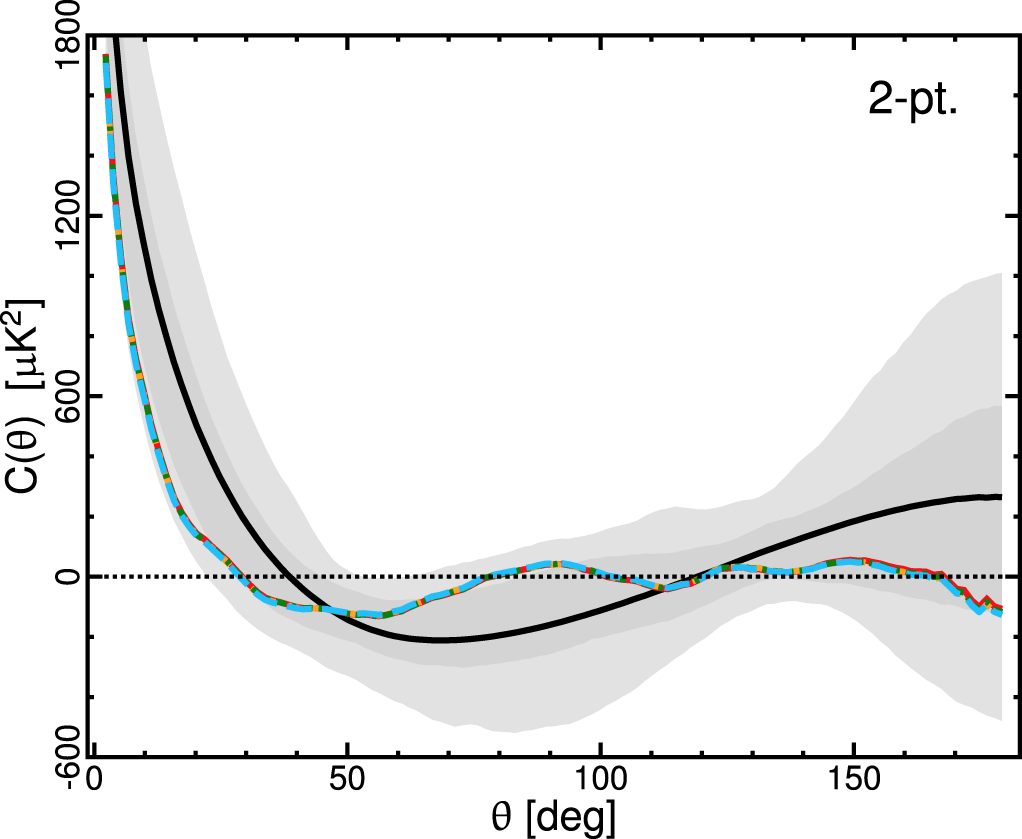