


ABSTRACT
We present a comprehensive data description for Ks-band measurements of Sgr A*. We characterize the statistical properties of the variability of Sgr A* in the near-infrared, which we find to be consistent with a single-state process forming a power-law distribution of the flux density. We discover a linear rms–flux relation for the flux density range up to 12 mJy on a timescale of 24 minutes. This and the power-law flux density distribution implies a phenomenological, formally nonlinear statistical variability model with which we can simulate the observed variability and extrapolate its behavior to higher flux levels and longer timescales. We present reasons why data with our cadence cannot be used to decide on the question whether the power spectral density of the underlying random process shows more structure at timescales between 25 minutes and 100 minutes compared to what is expected from a red-noise random process.
Export citation and abstract BibTeX RIS
1. INTRODUCTION
Sagittarius (Sgr A*), at the center of the our Galaxy, is a highly variable near-infrared (NIR) and X-ray source which is associated with a 4 × 10⁶M☉ supermassive central black hole (Eckart & Genzel 1996, 1997; Eckart et al. 2002; Schödel et al. 2002; Eisenhauer et al. 2003; Ghez et al. 1998, 2000, 2005b, 2008; Gillessen et al. 2009). While first detected as a bright, ultracompact, and comparatively steady radio source, the strong variability at shorter wavelengths, the variable polarization of the NIR emission, and the correlation between fluctuations in the submillimeter, NIR, and X-ray regimes provide evidence that this variable emission originates in the direct surroundings of the black hole. Therefore, properties of the black hole and of the emission and accretion mechanisms in its close surroundings can be studied at these wavelengths (Baganoff et al. 2001; Porquet et al. 2003, 2008; Genzel et al. 2003; Ghez et al. 2004, 2005a; Eckart et al. 2004, 2006a, 2006c, 2006b, 2008a, 2008b, 2008c; Yusef-Zadeh et al. 2006a, 2006b, 2007, 2008; Hornstein et al. 2007; Dodds-Eden et al. 2009; Sabha et al. 2010).
To explain the observed variability and its correlation between the NIR and X-ray regimes, several authors suggest synchrotron self-Compton (SSC) or inverse Compton emission as the responsible radiation mechanisms (Eckart et al. 2004, 2006a, 2006c; Yuan et al. 2004; Liu et al. 2006; Eckart et al. 2012). Relativistic models that assume the variability to be linked to emission from single or multiple hot spots in the accretion disk near the last stable orbit of the black hole have been applied successfully to individual data sets (Meyer et al. 2006a, 2006b, 2007; Zamaninasab et al. 2008). These models interpret the shorter timescales of the variability (between 10 and 30 minutes) to be dominated by the orbital motion.6 Orbital motion close to the black hole (and an associated quasi-periodic signal in the light curves) is of special interest: it could be used as a timing experiment in a strong gravitational field that might allow for determining black hole parameters like spin or inclination.
Potential quasi-periodic oscillations (QPOs) have been found in some light curves (see, e.g., Genzel et al. 2003). However, these QPOs are not statistically significant within the overall variability. Based on NIR light curves from seven nights of observing with the Keck telescope, Do et al. (2009) analyzed the flux density distribution of Sgr A* and the significance of quasi-periodic oscillations. They showed that QPOs in total intensity light curves cannot be established with sufficient significance against random fluctuations, finding a pure red-noise power spectral density (PSD) sufficient to account for the time correlation of the fluctuations.
On the other hand, based on relativistic models, Zamaninasab et al. (2010) predicted a correlation between the modulations of the observed flux density light curves and changes in polarimetric data (also see Eckart et al. 2006a; Meyer et al. 2006a, 2006b, 2007; Eckart et al. 2008a; Cunningham & Bardeen 1973; Stark & Connors 1977; Abramowicz et al. 1991; Karas & Bao 1992; Hollywood et al. 1995; Dovčiak et al. 2004, 2008). A comparison of predicted and observed light curve features (obtained from six nights of polarimetric observations with the Very Large Telescope (VLT) and the Subaru telescope) through a pattern recognition algorithm resulted in the detection of a signature possibly associated with orbiting matter under the influence of strong gravity.
Since the first discovery of the variable emission of Sgr A* in the NIR in 2003 (Genzel et al. 2003), a number of publications have concentrated on the statistical properties of the flaring activity rather than on interpreting individual observations. These papers investigated the timing properties of the light curves as well as the radiation mechanisms involved (Yusef-Zadeh et al. 2009; Zamaninasab et al. 2010; Bremer et al. 2011; Schödel et al. 2011; Eckart et al. 2012). On the basis of 14 light curves observed between 2004 and 2008, including alternating observations with VLT and Keck, Meyer et al. (2009) first discovered a dominant timescale at about 150 minutes, supporting linear scaling relations of break timescales in the PSD with black hole mass. They determined the power-law slope of the high-frequency part of the PSD to be 2.1 ± 0.5.
A comprehensive statistical approach in the analysis of the Ks-band total intensity variability observed with NACO at the VLT has been conducted by Dodds-Eden et al. (2011). The authors analyzed VLT K-band data between 2004 and 2009. They presented a detailed investigation of the flux density statistics and described the time-variable stellar confusion at the position of Sgr A* which makes an investigation of the faint emission difficult. They also emphasized the importance of these faint states for the overall statistical evaluation of the variability of Sgr A*. Based on the flux density histogram, the authors claim evidence for two states of variability, a log-normal-distributed quiescent state for flux densities <5 mJy and a power-law-distributed flaring state for flux densities >5 mJy. They argue that it is very unlikely that the same variability process is responsible for both high and low flux density emission from Sgr A* (the statistical model the authors promote is summarized in Appendix A). With reference to this model, Genzel et al. (2010, p. 3176) state that "it is a key issue whether the brightest variable emission from Sgr A* [is] statistical fluctuations from the probability distribution at low flux or flare events with distinct properties" and that "the transition from the log-normal distribution at low-flux levels to the tail of high fluxes may also explain the apparent mismatch between the detection versus non-detection of quasi-periodic substructures in different near-infrared light curve studies (p. 3179)."
Our statistical analysis presented in this paper serves the following goals:
- 1.to provide a more comprehensive, uniformly reduced data set of Ks band observations from 2003 to early 2010;
- 2.to conduct a rigorous analysis of the observed flux density distribution;
- 3.to explain why a proper statistical analysis of the Ks-band light curves cannot reproduce the results found by Dodds-Eden et al. (2011);
- 4.to conduct a rigorous time series analysis on the basis of a representative data set;
- 5.to propose a comprehensive statistical model that, using standard methods for generating Fourier-transform-based surrogate data, describes all aspects of the observed (total intensity) data and lets us simulate light curves with the observed time behavior and flux density distribution;
- 6.and to investigate extreme variability events in the context of our statistics.
2. DATA REDUCTION
In the following, we describe the data and the reduction methods we applied in order to obtain time-resolved photometric information on Sgr A*. Whereas large portions of the data set are the same as used in the analysis by Dodds-Eden et al. (2011), we have chosen different reduction methods: Lucy–Richardson (LR) deconvolution in order to guarantee the best possible isolation of the target sources from nearby point-like sources, a well-controlled flux density calibration with 13 stars, and an objective quality cut based upon seeing and Strehl ratio values.
2.1. The Data Set
Our analysis is based on ESO archive data. All observations have been conducted with the NIR adaptive optics (AO) instrument NAOS/CONICA at the VLT in Chile (Lenzen et al. 2003; Rousset et al. 2003). We included all available Ks-band frames of the central cluster of the Galactic center (GC) from early 2003 to mid-2010. For all observations, the NIR wavefront sensor of the NAOS AO system was used to lock on the NIR bright supergiant IRS 7 (variable,  = 6.5 in the 1990s,
  = 7.4 in 2006, and
  = 7.7 in 2011, 5
 6 north of Sgr A*7). Two different cameras, S13 and S27, with 13'' and 27'' fields of view,8 respectively, and a polarimetric mode with inserted Wollaston prism and mask have been used. The small field of view of the polarimetric mode restricted the set of calibrators to the innermost arcsecond around Sgr A*.
We concentrated on data sets with a length of more than 40 minutes (shorter data sets are often severely affected by bad weather conditions in which case the observer decided to change to another wavelength or target). Problematic frames with obviously bad AO-correction (most of the stars not visible at all) or frames, which do not show Sgr A* or a sufficient number of calibrators, have not been included for the photometric analysis. Ultimately we investigated 12,855 frames photometrically. Table 2 shows a list of all data sets that are part of this analysis.
2.2. Data Reduction and Flux Density Calibration
We performed every reduction step for every frame uniformly: the reduction included basic steps like sky subtraction, flat fielding, and correction for bad pixels. For total intensity data, we used sky flat fields (where available), for polarimetric data, we used a lamp flat field (Witzel et al. 2011). Most of the data were observed using a jitter routine with random offsets to prevent systematic influences on the measurements by detector artifacts. These offsets need to be detected and corrected for to guarantee stable aperture photometry at a constant position. This was achieved with a cross-correlation algorithm for sub-pixel accuracy alignment (ESO Eclipse Jitter; Devillard 1999). For each aligned frame, we determined an estimate of the point-spread function (PSF) with the IDL routine Starfinder (Diolaiti et al. 2000) using separated stars like S30 or S65 in the 2'' surrounding of Sgr A*. The PSF-fitting algorithm of Starfinder provided an estimate of the extended background in each single frame and a list of detected stars with position and relative flux density. We decided not to use the values resulting from Starfinder photometry (for a detailed reasoning see below). Instead we used the LR deconvolution algorithm to separate neighboring point-like sources. In the case of polarization data, we aligned all (4–6) polarization channels of the individual observation night with the cross-correlation algorithm. Data observed with the different pixel scale of the S27 camera (002715) were resampled to 001327 (S13). Finally, a beam restoration was carried out with a Gaussian beam of an FWHM corresponding to the diffraction-limited resolution at 2.2 μm (∼60 mas).
After the preparative steps described we conducted aperture photometry at the position of 13 constant calibrators (Rafelski et al. 2007), of 6 comparison stars, at the position of Sgr A*, and at 8 positions where no star was detected (B- and C-apertures), to measure the background flux (see Figure 1). The background was estimated at the locations of lowest background (six apertures) and close to Sgr A* (two apertures) where no obvious point-like source is visible. We applied a circular masking of radius 004 at all the measurement positions. For a small number of observations, according to the available field of view, we accepted a smaller set of calibrators (at least seven).

Figure 1. Ks-band image from 2004 September 30. The red circles mark the constant stars (see variability study in Rafelski et al. 2007) which have been used as calibrators, the blue the position of photometric measurements of Sgr A*, comparison stars, and comparison apertures for background estimation. Source identifications from Gillessen et al. (2009).
Download figure:
Standard image High-resolution imageThe positions of the apertures in each night have been defined as consistently as possible: for Sgr A* with the help of its brighter states, for the stars with the help of mosaics (averages over the single frames of one night in order to increase the signal-to-noise and to also estimate the centroid of the fainter comparison stars), carefully following their proper motions. For the background apertures and the aperture of Sgr A* when it was faint we conducted triangulation relative to nearby stars. Then one set of positions was used for all frames of the corresponding night. For some polarimetric observations NACO was rotated. In these cases, we determined a rotation matrix for the position coordinates, making them comparable to the closest unrotated observations.
For each aperture, we summed up its total content in analog-to-digital units (ADU). For the polarimetric data, the ADU values obtained for orthogonal channels were added. We subtracted the average background value (B-apertures) in ADUs from the calibrator values and conducted a flux density calibration using the photometric values for the calibrators in Table 1 (Schödel et al. 2010). Because of the high proper motions of the stars within this field, the state of confusion of the calibrators changes from epoch to epoch. We applied the following algorithm to reduce the epoch-dependent systematic error of the calibration.
Table 1. List of Calibrators
| Star |  |
Flux Density |
|---|---|---|
| (mJy) | ||
| S26 | 14.94 | 6.79 |
| S27 | 15.41 | 4.41 |
| S6 | 15.35 | 4.66 |
| S7 | 14.92 | 6.92 |
| S8 | 14.21 | 13.31 |
| S35 | 13.20 | 33.74 |
| S10 | 13.95 | 16.91 |
| S65 | 13.58 | 23.78 |
| S30 | 14.12 | 14.46 |
| S98 | 15.27 | 5.01 |
| S100 | 15.29 | 4.92 |
| S84 | 14.66 | 8.79 |
| S107 | 14.82 | 7.59 |
Note. The flux density for each star was calculated correcting for extinction with mext = 2.46.
Download table as: ASCIITypeset image
First, for each calibrator k we calculated the quantity:

with ck being the background-subtracted ADU values for the kth calibrator and mref its reference magnitude. We sorted these values, rejected the three largest and the three smallest values (for the data sets with less calibrators we accordingly reject a smaller number), and took the arithmetic average f0 over the remaining values. According to Tokunaga (2000), we then obtained the magnitude mA and flux density FA for each aperture A by

with mext = 2.46 being the K-band extinction as determined in Schödel et al. (2010). This procedure ensures a best possible constance of the flux density calibration under the changing conditions of each data set.
As a last step, we collected parameters for each frame that provide information on the data and calibration quality, which allowed us to reject data points based on objective criteria. These parameters are: Julian date, integration time (NDITxDIT), rotator position angle (orientation of NACO), airmass, FWHM of the active optics guide star PSF, coherence time of the atmosphere, camera, all obtained from the header of the fits data, and the number of stars detected by Starfinder, the Strehl ratio calculated from the extracted PSF using the ESO Eclipse routine STREHL, the rms of the values fk, and, as the most important quality check, the average normalized flux of the calibrators. This last quantity is obtained for each frame by dividing the measured flux density of the individual by its reference value and averaging over all available (i.e., not rejected) calibrators.
We emphasize that both methods—PSF-fitting and LR aperture photometry—are in general equivalent for estimating the flux density of a point source (Meyer et al. 2008). However, in the case of the presence of extended flux underlying a dim and confused point source observed under varying correction performance of the AO-system, it is more difficult to control
- 1.how Starfinder divides the given flux at a position into background and point-source flux,
- 2.how the possible overestimation of the flux due to noise-peaks influences the statistics of low flux densities (if the center of the fit is not forced to a given position), and
- 3.what non-detections due to the quality thresholds set in Starfinder mean for the overall statistics.
Also LR deconvolution has drawbacks, especially in handling extended flux that is added to existing point sources or gathered into artificial sources by the algorithm. We can account for this effect with a suitable big aperture and by monitoring apertures at positions without obvious point sources. Thus, the statistics of the interplay between the background (coming from unresolved sources, truly extended emission, and PSF contributions from the surrounding point sources), the AO and point-like flux at a given position is directly propagated to the statistics of the measured values, which is crucial for understanding the instrumental influence on our flux density statistics and our statistics do not suffer from non-detections that might introduce a selection effect. We will come back to the measurement statistics in Section 3.
2.3. Light Curves of Sgr A*
As a result of the reduction procedure described in Section 2.2, we obtained the data shown in the upper panel of Figure 2. For convenience and following the visualization used in Dodds-Eden et al. (2011), we show a concatenated light curve with all time gaps longer than 30 minutes reduced to the average sampling of the individual data sets (1.2 minutes). This visualization shows the data of all nights as a pseudo-continuous light curve allowing for a comparison of the variability and the confusion in each epoch. A visualization of the true cadence is presented in Section 4. The timing analysis in Section 4 is based on the true cadence and not on the concatenated light curve.

Figure 2. Concatenated light curve of Sgr A* and S7 with time gaps longer than 30 minutes reduced to 1.2 minutes. The top panel shows the result of aperture photometry before the quality cut, the next panel the same data after quality cut and removal of offsets. The third shows a light curve of S 7, a nearby star that has been used as a calibrator. The time gaps are the result of the rejection procedure described in Section 2.2. The lower panel shows the average ratio between the measured flux of each calibrator and its reference value (Table 1), scaled with a factor of 15. Its noise corresponds to the error a hypothetical noise-free aperture with a flux density of 15 mJy would have only due to the uncertainties of the calibrators.
Download figure:
Standard image High-resolution imageThese 12,855 data points still include points of bad observation conditions and insufficient calibration reliability. We used an objective frame rejection algorithm by incorporating information on seeing, Strehl ratio, fraction of stars detected by Starfinder,9 the standard deviation of the f0-values obtained from the individual calibrators in each frame, and the normalized average calibrator flux density as described in Section 2.2. Only frames with seeing <2'', a Strehl-ratio >6%, an f0-standard deviation <16% of the average f0-value, and a normalized average calibrator flux density between >0.96 and <1.04 have been accepted.
The top panel of Figure 2 additionally shows a long-time trend of the data from epoch to epoch. As far as these "offsets" are concerned we agree with the conclusions of Dodds-Eden et al. (2011) that confusion with stellar sources is responsible for this long-term trend in a first approximation. In order to make the different years comparable, we subtracted the 2.5 percentile value of the flux in each epoch, resulting in 0 mJy for 2003, 0.3 mJy for 2004, 1.0 mJy for 2005, 1.0 mJy for 2006, 1.3 mJy for 2007, 2.8 mJy for 2008, 2.1 mJy for 2009, and 0.7 mJy for 2010. In 2003 and 2004, Sgr A* could be sufficiently separated from the near star S210 by the deconvolution reduction step.
The second panel of Figure 2 shows the data after quality cut and subtraction of the faint stellar contribution. For comparison and as an indicator of the calibration stability we show additionally the light curve of one of the calibrators, S7, in the third panel, and, in the lowest panel, the average calibrator flux density scaled to 15 mJy. On average, the calibration is very stable and the data points after quality cut exhibit a relative standard deviations of the average calibrator flux of 1.4%.
For a more detailed inspection, we present 112 data blocks (defined by continuity without gaps of more than 30 minutes) in Appendix C.
3. STATISTICAL ANALYSIS OF THE FLUX DENSITY DISTRIBUTION
In this section, we investigate the properties of the flux density statistics of the variability of Sgr A*. This analysis gives information on both the intrinsic flux density distribution of the variability as well as the instrumental effects within our measurements. The differentiation between instrumental features within the distribution and the intrinsic component turns out to be crucial in the context of the question of whether the intrinsic flux density distribution provides evidence for two physical mechanisms at work. Additionally, this analysis allows us to develop a full statistical model of the variability of Sgr A* in the next section.
3.1. Optimal Data Visualization
The first step in the analysis of the flux density distribution of Sgr A* is a proper graphical representation of the data in the form of a histogram. A representation of our data in a simple flux density histogram, normalized by the total number of points and bin size, is shown in Figure 3.

Figure 3. Flux density histogram of Sgr A*, based on the data shown in Figure 2.
Download figure:
Standard image High-resolution imageTo investigate the high flux density tail of this distribution, a logarithmic histogram with an equally spaced logarithmic binning is best suited. The number of bins for a given data range is a crucial parameter for the evaluation of the structure of the sample distribution. Following the study of Knuth (2006), we first determine the best bin size. As the author points out, the idea is to choose a number of bins sufficiently large enough to capture the major features in the data while ignoring fine details due to random sampling fluctuations. By considering the histogram as a piecewise-constant model of the probability density function from which n data points xi were sampled the author derives an expression for the relative logarithmic posterior probability (RLP) for each bin number:

with N being the number of bins and nλ the value of the λth bin. To find the best number of bins M, the posterior probability has to be maximized:

The best estimator for the bin value μλ and its variance σ2λ given the bin values nλ is deduced to be

and

with v being the interval between the maximum and the minimum measurement value.
Knuth (2006) demonstrates in his study that these results outperform several other rules for choosing bin sizes, e.g., "Scott's rule" or "Stone's rule."
We applied the described binning method to our data for Sgr A*. To make the flux density distribution comparable to the results by Dodds-Eden et al. (2011), which include the flux density of the star S17 due to a double aperture method, we added 3 mJy to the flux density of Sgr A*. We find a best bin number of M = 32. The dependence of the log posterior on the bin number is shown in Figure 4. The best piecewise-constant model (i.e., an estimator of the best histogram representation) describing our sample is shown in Figure 5. The histograms in this work have been created using this method.

Figure 4. Optimal data-based binning. We show the log posterior probability as a function of the number of bins. The maximum for the logarithmic flux density of Sgr A* is reached for 32 bins (blue line). The black lines represent bin numbers used for the histograms in Appendix D which clearly show that our results do not strongly depend on the binning.
Download figure:
Standard image High-resolution image
Figure 5. Best piecewise-constant probability density model for the flux densities of Sgr A*. The red error bars are the uncertainty of the bin height for the full 10,639 data points. The second bin height visible in some cases and the black error bars belong to the average histograms of 1000 data sets with 6774 data points (Dodds-Eden et al. 2011), generated by randomly removing points from our full data set. The overplotted cyan and magenta dashed lines show the log-normal distribution and the power-law distribution found in the analysis by Dodds-Eden et al. (2011), the blue lines show the combined distribution of those components, convolved with a Gaussian with a flux-density-dependent σ (compare Equations (A1)–(A4)).
Download figure:
Standard image High-resolution imageAdditionally, to the best histogram model obtained from Equations (5) and (6), we overplotted a graph of the model11 proposed by Dodds-Eden et al. (2011). It is obvious that our sample is more populated in the middle flux density range between 7 mJy and 15 mJy and shows a linear behavior between 4 mJy and 17 mJy, not showing any break or change of slope. That the shape of our histogram is not sensitive to the binning is shown in Appendix D where we present histograms with 22 bins for the range of the observed flux density values (resulting in a comparable bin width as used by Dodds-Eden et al. 2011) and 45 bins,12 both reproducing the linear trend. Rather than being a matter of representation, this difference is related to the different sample selection (10,639 data points in this work in comparison to 6774 points in the case of Dodds-Eden et al. 2011). To better understand the character of the selected subsample in Dodds-Eden et al. (2011; their quality cut is based on the visual impression of the individual frame), we randomly selected 6774 points from our sample (by nonparametric bootstrapping, i.e., sampling with replacement) and generated 1000 surrogate data sets in this way, binned each data set in a histogram with the same bin size as that of our total sample, averaged the bin values over all surrogate sets, obtained an error from the standard deviation, and plotted the result as the second bin height (now with black error bars) in Figure 5. One can clearly see that for most of the bins there is barely any difference, showing that a random influence cannot be responsible for the difference of both distributions. This test also shows the robustness of the linear behavior of the histogram in the case of smaller data sets under random selection. Furthermore, in our data set we do not see the observation conditions to be correlated with the flux density states of Sgr A* (compare Figure 2 and Appendix B). In general, data worse than average should also be represented in the uncertainties, and not simply eliminated, because otherwise errors might be underestimated due to an introduced bias, and we have to conclude here that the subsample used by Dodds-Eden et al. (2011) shows a severe selection effect.
The linear behavior in the log–log diagram points toward a power-law distribution p∝x−α as a possible description for all flux densities higher than ∼4 mJy. The statistical significance of this visual impression is analyzed in the next section. We mention here that a power-law distribution is only showing a linear behavior in a log–log diagram if it is of the form

Otherwise, the logarithm log (p) of the probability density is only linear as a function of log (x) for large values of x:

This is the main reason why the distribution claimed in Dodds-Eden et al. (2011) shows a break. In this case the high flux density tail is described by a power law with x0 ≈ 0.8 mJy, and this power law does not show a linear behavior in the log–log diagram if plotted versus the sum of the intrinsic flux density, background, and the flux density of S2. It starts to deviate from a linear behavior (it, so to say, "breaks") close to the transition value Ft of the total distribution (see Figure 5, blue and magenta dashed lines). Thus, even if we accept the selection of data points by Dodds-Eden et al. (2011), the visual impression of the necessity of introducing a break in the distribution is a feature of the data visualization, and in their case the power law is also actually suited to describing the data down to a flux density value of about 4 mJy quite well. This means, even under the assumption that the data selection of Dodds-Eden et al. (2011) is valid, the discussion of a double state model for Sgr A* and its significance is very much dependent on the evidence of a log-normal model describing the low flux density part of the histogram. We come back to this point in the next section.
The reason why we see the distribution behaving linearly in our visualization is a coincidental equality of −x0 = 3 mJy in our power-law model (see next section) and the flux density of S17 (≈3 mJy) which we added to the flux density of Sgr A* to make it comparable with the distribution proposed by Dodds-Eden et al. (2011).
3.2. Power-law Representation of the Intrinsic Flux Density Distribution
We begin with a description of the instrumental effects and uncertainties of our photometry. Figure 6 shows the flux density histograms of 10 stars (calibrators and comparison stars). As expected, the width of the distribution decreases with decreasing flux density of the source. To estimate the FWHM of the scatter of our photometry at a given flux density, we fit Gaussian distributions to the histograms. The σ values of these fits as a function of the mean flux density are shown in Figure 7. For our photometry we clearly find smaller uncertainties than Dodds-Eden et al. (2011) for their aperture photometry, very similar to their Starfinder photometry, or the photometry of Do et al. (2009). In contrast to Dodds-Eden et al. (2011), the functional dependency shows a clear flattening toward small flux densities13 and we cannot confirm the dominance of photon noise (Dodds-Eden et al. 2011). We find a parabola to be a suited (phenomenological) description up to flux densities of 32 mJy. Actually, the uncertainties in the flux density range between 0 and 10 mJy are more or less constant. This corresponds well to the visual impression that the variable AO-correction and its influence on the background contribution due to PSF halos of bright sources (halo noise; Fritz et al. 2010) as well as differential tip/tilt jitter and their interplay with the deconvolution are the dominant reasons for the uncertainties.

Figure 6. Normalized flux density histograms of 10 calibration stars. The dashed curves are Gaussian fits to the flanks of the distribution, suppressing the broader tails of the distributions. This guarantees a proper measurement of the FWHM of the distributions.
Download figure:
Standard image High-resolution image
Figure 7. Measurement error as a function of flux density. The purple line is a quadratic fit to the measured σ values of the calibration stars shown in Figure 6 (blue crosses). The red line is the power-law dependency found by Do et al. (2009) for their data, the green line and the black line the dependency found by Dodds-Eden et al. (2011) for their aperture photometry and their PSF-fitting photometry, respectively. The two magenta crosses represent the measured σ values at the position of the C-apertures, compare Figure 1.
Download figure:
Standard image High-resolution imageThe role of halo noise becomes evident when looking at the control apertures close to Sgr A* (Figure 1, C-apertures). Their average flux density is clearly not zero, and the flux density values are scattered around the mean with an FWHM comparable to the width of all flux density distributions of the stars fainter than 10 mJy. The aperture west of Sgr A* shows a varying contribution of faint confusion on the level of a few tenths of a mJy (Figure 8, blue histogram). The average flux density of these "empty" apertures is about 0.6 mJy.

Figure 8. Flux density histograms of the two background (C-) apertures (blue, brown) close to Sgr A* in comparison to the flux distribution of Sgr A* (magenta). The dashed curves are Gaussian fits to the flankes of the distributions.
Download figure:
Standard image High-resolution imageIn the following, we investigate if a power-law distribution indeed is suited to describing our sample. We follow the strategy described in Clauset et al. (2007) for identifying power-law distributions and determining their parameters. The authors of this study point out that a least-squares regression to a histogram in log–log representation can generate significant systematic errors, mainly due to the non-Gaussianity of the variation of the logarithmic bin height. Furthermore, binning the data in a histogram introduces further parameters corrupting standard goodness-of-fit estimators. The procedure described in the following overcomes this problem.
The probability density of a power-law distribution is defined as

with xmin = xmin, intr − x0 and xmin, intr being the lowest value to which the data are power-law distributed, making the power-law normalizable with a normalization factor (α − 1) · xα − 1min. The corresponding cumulative distribution is given by

The steps for analyzing power-law-distributed data are as follows (Clauset et al. 2007).
- 1.Find estimators for xmin and x0 and the maximum likelihood estimator for α. The maximum likelihood estimator for α given any value for xmin and x0 is calculated using the equations
 with x > xmin + x0 and ntail being the number of data points higher than xmin + x0. Estimators for xmin and x0 are obtained by choosing xmin and x0 in a way that makes the probability density and the best-fit power-law model (i.e., the power law with α as the maximum likelihood estimator) as similar as possible. The similarity is estimated by Kolmogorov–Smirnov (K-S) statistics:with P(x) being the cumulative distribution of the best-fit power-law model and C(x) the relative cumulative frequency of the empirical data sample. The parameter D has to be minimized. The error on xmin and x0 can be found by a nonparametric "bootstrap" method, i.e., (given n empirical data points) by drawing a new set of n data points uniformly at random from the empirical data and determining the standard deviation of xmin and x0 for these surrogate samples. To replicate the act of drawing an independent, identically distributed sample from the population the surrogate data have to be drawn with replacement.
 - 2.Test for plausibility by calculating the goodness of fit between the empirical data and the power law. The goodness-of-fit parameter q is defined as the fraction of synthetic data drawn from the best-fit probability model that has worse K-S statistics than the empirical data sample. Here it is important to obtain the K-S value D for each synthetic sample in the same way as for the empirical data, i.e., the estimators for xmin, x0, and α have to be found for each synthetic sample individually and the K-S value has to be calculated relative to the individual best-fit power law. To ensure that the xmin values are determined under the same conditions as for the empirical data sample we have to make sure that the synthetic sample follows the empirical data sample distribution for the values smaller than xmin + x0. This is realized by choosing with probability 1/ntail a random number from the best-fit empirical power law and with probability 1 − 1/ntail a value from the empirical data below the xmin + x0 estimate (with ntail being the number of data points higher than xmin + x0). A q-value >0.05, or more conservative >0.1, makes the power-law model a plausible assumption.


With a simulation of 1000 surrogate samples (again obtained by nonparametric bootstrapping) for determining the errors of xmin and x0 and 6000 synthetic samples for testing for plausibility we obtained the values:

A goodness-of-fit parameter q = 0.2 means that in a fifth of the cases a sample drawn from a power law with parameters as in Equation (14) will show deviations worse than our empirical sample, making the power-law description plausible for all flux densities higher than 4.2 mJy (note that the exact value of x-axis offset is x0 = −2.9 mJy, close to the value found due to the linear appearance of the histogram in the log–log diagram). A diagram of the cumulative distribution function (CDF) of the best-fit power law and the empirical relative cumulative frequency is shown in Figure 9. For a comparison, we also overplotted the CDF of the model proposed by Dodds-Eden et al. (2011; restricted to flux density values higher than xmin). Figure 10 shows the value of the power-law slope α as a function of xmin. As expected, the best xmin is close to the point where α starts to be constant for a range of xmin values (compare Figure 3.3 in Clauset et al. 2007).

Figure 9. Estimation of the goodness parameter p by a Kolmogorov statistic. The value p is defined by the maximum difference of the measured CDF (black) with respect to the CDF of the best fitting power law (red). In green, we show the CDF of the model proposed by Dodds-Eden et al. (2011) restricted to flux density values higher than xmin.
Download figure:
Standard image High-resolution image
Figure 10. Scaling parameter α as a function of the value for xmin (compare Figure 3.3 in Clauset et al. 2007).
Download figure:
Standard image High-resolution imageEquation (11) only represents the maximum likelihood estimator for the power-law slope if the xi are independent or at least uncorrelated, otherwise the estimator is biased. However, we know that for our sample the xi are not uncorrelated, since the flux densities are occurring in "flares," it means in a time-continuous development. This simply describes the fact that finding the flux density to be at a level of 15 mJy implies very low probability for a level of 5 mJy to be reached within, e.g., the next 3 minutes. This predictable behavior disappears on longer timescales, and it is not possible anymore, knowing the flux density at a time point t0, to predict the flux density level, e.g., 100 minutes later, very reliably. This has been investigated by Meyer et al. (2009) in their analysis of the PSD discovering a timescale of about 150 minutes. Here we are analyzing data covering about 15,000 minutes, a hundred times longer than the timescale on which the correlation of the data vanishes. This means to first order and because the estimator in Equation (11) is most sensitive to data points close to xmin (where the histogram is most populated and the value of each bin can be considered to be fairly independent from the neighboring bins), the bias is negligible. For the high flux density tail the bias due to the time correlation is significant because here the histogram bars are populated only with data points of the rare strong outbursts. In the case of our data set, all histogram bars higher than about 17 mJy are populated only due to one very bright outburst. This is the reason why for higher flux densities the empirical cumulative distribution deviates more from the ideal CDF of the model and the statistics become incomplete. This effect is also visible in Appendix D, where we show the ideal CDF, the empirical cumulative distribution, and the cumulative distribution of some of the uncorrelated synthetic samples we generated for the estimation of the goodness parameter q. For high flux densities, many synthetic data sets show a closer development with respect to their best-fit CDF than our empirical sample, even if their K-S value D is worse. In this context, it is important to note that the synthetic samples with a worse K-S statistic may differ significantly from the ideal CDF at lower flux density ranges which is not well visible in a log–log diagram (see Appendix D). These arguments also show that a χ2-minimization fitting to the histogram is questionable, especially if the χ2-values are used to establish the significance of a distribution break based on the highest, most correlated bins.
Up to this point we found a description for flux densities higher than xmin. We can show that our data sample is consistent with a pure power law describing the intrinsic flux density distribution under the influence of an instrument with limited resolution and sensitivity and that xmin can be interpreted as the detection limit of NACO for Sgr A* due to being embedded in extended flux and its confusion from faint unresolved stars. The argument is simple. If we weight the power-law distribution for fluxes higher than xmin, with a factor ntail/n with ntail the number of data points with values higher than xmin, we can extend the power law to smaller flux densities until its integral becomes unity:

In our case, with the values of Equation (14) we find x*min = 3.57 ± 0.1 mJy. Correcting this value for x0 = −2.94 ± 0.1 mJy, this power-law distribution shows a cutoff at x*min + x0 = 0.63 ± 0.15, which is identical to the average flux density of the two background apertures close to Sgr A*. The measured distribution now can indeed be obtained by convolving the power-law distribution with a Gaussian distribution to account for the uncertainty of the photometry:

with σ* being the half-width at half-maximum of the error distribution, which for our data sample can be considered constant up to ≈15 mJy (see Figure 7). For higher values the histogram starts to be incomplete, and the bias due to the time correlation is dominating the statistical errors. The slope of the power law is slightly changed by the convolution, but for values of σ* of the magnitude of the observational errors this effect is within the errors of α.
By using K-S statistics again we find a constant value of σ* ≈ 0.32 mJy as a best fit to the histogram (see Figure 11). This value is larger than the observed error σ* ≈ 0.2 mJy of better separated sources (see Figure 7). The reason is that the photometry on Sgr A* for a large fraction of the data is influenced by the nearby star S17, and that we subtracted a constant offset from epoch to epoch, for which it is difficult to find a realistic error. Both influences effectively broaden the expected distribution (which, as a result, is not Gaussian anymore, but somewhat less peaked) that this is not a disadvantage of the deconvolution method with respect to the double aperture method preferred by Dodds-Eden et al. (2011) can be seen in Figure 7. The error of the double aperture photometry for the low flux density range of Sgr A* (starting at flux densities >3 mJy) is also in the range of >0.3 mJy.

Figure 11. Flux density histogram as in Figure 5. The blue line shows the extrapolation of the best power-law fit; the cyan line shows the power law convolved with a Gaussian distribution with σ = 0.32 mJy.
Download figure:
Standard image High-resolution imageWe conclude that it is not possible to verify the evidence of an intrinsic turnover (that could indicate the peak shape of a log-normal distribution) based on the larger scatter of the low states of Sgr A* with respect to the typical error of a better separated source of this flux density. The difference of 0.1 mJy between the typical error of a faint source of 0.2 mJy and the error value for our best fit of 0.32 mJy is well within the uncertainties of our knowledge about the true error distribution at the position of Sgr A* as Figure 8 demonstrates. Having no evidence for a log-normal distribution for low flux density values,14 the necessity of a break in the distribution to account for the highest flux densities vanishes, even if we accept the data selection of Dodds-Eden et al. (2011) and ignore the fact that all flux density bins higher than 17 mJy are populated due to one bright event only. Rather than a double state description we prefer a simple power law with a slope of α = 4.2 ± 0.1 and an intrinsic pole at x0, intr. = x0 − backgr. = −x*min = −3.57 ± 0.1 mJy. Since flux density is a positive quantity, this intrinsic power law naturally breaks at x*min, intr. = x*min + x0, intr. = 0 mJy. The instrumental effects on the photometry are sufficiently described by a Gaussian distribution centered around the background value of 0.6 ± 0.1 mJy with a constant σ = 0.32 mJy. This instrumental effect leads to a detection limit, which here is defined as the limit up to which a reliable photometry is not possible, of ∼0.7 ± 0.16 mJy intrinsically, and ∼1.3 ± 0.15 mJy for the actual measurements which include the background flux density of 0.63 ± 0.15 mJy. With the power-law model, we find a median value for the flux density of med(x)intr. = 0.9 ± 0.15 mJy (corrected for the background) or med(x)obs. = 1.5 ± 0.1 mJy (including the background flux density). This shows that, assuming we can extrapolate the power law to smaller flux densities below the detection limit, we find the average flux density to be very close to the detection limit, indicating a severe limitation of the knowledge about the variability of Sgr A* we are able to infer from our data. The relation of x0, xmin, x*min and the background flux density is schematically shown in Figure 12.

Figure 12. Schematic view of the power-law flux density distribution and the parameters xmin, x*min, x0 and the background flux density (y-axis in arbitrary units, x-axis in mJy). We show the measured flux density distribution (gray area) after adding 2.94 mJy to account for x0, the pole of the measured non-shifted power law (which belongs to the non-shifted distribution indicated by the long-dashed line), and the intrinsic distribution with and without correction for x0 (described by the continuous lines ∝x−α and ∝(x − x0)−α, respectively). As in Equation (9), xmin is the minimum flux density down to which the shifted measured distribution is a power law, and x*min is the minimum flux density obtained by an extrapolation of the power law toward lower values, assuming the distribution below xmin to be dominated by instrumental effects. Therefore, x*min represents the intrinsic minimum flux density in the case of the x0-shifted distribution. For the case of the non-shifted distribution the intrinsic minimum is represented by x*min + x0, which equals the background flux density within our uncertainties. Thus, the intrinsic minimum x*min, intr. = x*min + x0 − backgr. (now additionally corrected for the background) equals zero.
Download figure:
Standard image High-resolution imageOf course we cannot prove that the flux density distribution is a strict power-law distribution. We only can show that the observable intrinsic flux densities can be well described by this model. This assumption is simpler and needs less parameters than the assumption of a broken distribution. Nevertheless, it might well be that the real distribution shows some structure at flux densities below the detection limit. In particular, it might even follow a log-normal distribution (with a high multiplicative standard deviation to account for the linear appearance in the log–log plot). The log-normal distribution used in the model of Dodds-Eden et al. (2011) and evidence for a break in the distribution at an observable flux density level, however, can be ruled out.
For the sake of comparability with other objects that show log-normal distributions (e.g., Gaskell 2004) we want to include here the best-fit parameters for a simple log-normal model. It is not easy to estimate the parameters (and their uncertainties) of a log-normal distribution describing the intrinsic flux. The reason is that due to the described instrumental effects we do not have precise knowledge about the shape and position of the intrinsic peak. This is a more severe restriction in the case of a log-normal model that is characterized by its intrinsic turnover than for the power-law model.15 Fitting the linear histogram with a log-normal model as defined in Equation (A4) convolved with a Gaussian (with the width of the Gaussian as a free parameter) we obtain a best fit for σ* = 1.00 ± 0.05, μ* = 0.12 ± 0.07, xb = 3.38 ± 0.15, a width of the Gaussian distribution of σ* = 3.38 ± 0.06, and a χ2/dof = 1.6. The given uncertainties are larger than the formal uncertainties. In particular, they allow for larger deviations from the histogram at low flux densities than implied by the statistical errors of the bin. This accounts for the fact that the true instrumental effects are only approximately Gaussian (due to the non-uniform white noise contribution each night and the epoch-wise correction for stellar confusion). The intrinsic median flux density of the log-normal model is 4.51 ± 0.2 mJy and equal to the corresponding value for the power-law model of 4.47 ± 0.2 mJy (both for the shifted distribution).
4. TIME SERIES ANALYSIS
In this section, we investigate the nature of the already mentioned time correlation of the flux density measurements. In a more formal description: assuming that all measurements are samples of the very same random process, and starting with the idea that this random process is (weakly) stationary (for which the impression of a stable mean and variance is indicative), we consider the flux density distribution of Section 3 as the marginal probability distribution of the random process. Now we want to find a characterization of the joint probability distribution. Whereas in general "red-noise" light curves16 can only be considered as weakly non-stationary, the (weak) stationarity for the underlying random process is a consequence of the PSD break found by Meyer et al. (2009) which is far shorter than the covered time period of 15,000 minutes.
A first, very simple approach for characterizing the time behavior of the variability is the following: let us associate the average sampling (of the concatenated light curve) of ∼1.2 minutes to every data point. In this way, we can relate the total time the source spent in the range of a given flux density bin to the total time covered by observations (∼15, 000 minutes), and we get a rough estimator for the fraction of time the source spends at that flux density. For a more detailed analysis we have to use standard time series analysis tools, like periodograms as estimators for the PSD of the process, Lomb–Scarle periodograms, the autocorrelation function, or the structure function (Scargle 1982; Priestley 1982; Simonetti et al. 1985). As Meyer et al. (2009) point out the given window function (covering ∼3.6 × 10⁶ minutes with a coverage fraction of only ∼0.4%) makes standard Fourier transform techniques unsuitable (see Figure 13). Similarly the Lomb–Scargle periodogram, generally suitable as a PSD estimator for non-equally sampled data, is based on the average sampling, which in this case is >3000 minutes. Do et al. (2009) used the approach of comparing and averaging the Lomb–Scargle periodograms of data subsets with similar length and sampling to access the PSD of the higher frequencies. In our case this approach again would probably introduce selection effects, and we decided to generally follow the method presented by Meyer et al. (2009), a Monte Carlo (MC) approach, similar to the PSRESP method by Uttley et al. (2002). Dodds-Eden et al. (2011) mention that the MC simulation approach used in Do et al. (2009) and Meyer et al. (2009) are based on a comparison sample with a flux density distribution that is Gaussian, and in particular allows negative values, questioning the validity of the method. In the following, we overcome these concerns by developing an algorithm that allows us to simulate time series with the flux density distribution we observe.

Figure 13. Light curve of Sgr A* as in Figure 2. In this case no time gaps have been removed; the data are shown in true time coverage. A comparison of both plots shows: only about 0.4% of the 7 years have been covered by observations.
Download figure:
Standard image High-resolution image4.1. rms–flux Density Relation
For the study of X-ray binary variability (linear), rms–flux relations represent an important piece of information. A relation between rms and the radiation flux was initially discovered in observations of black-hole and neutron-star X-ray binaries (Uttley & McHardy 2001). Since then the rms–flux relation has been studied in several other observations of black-hole binaries, active galactic nuclei (AGNs), neutron-star X-ray binaries, and ultraluminous X-ray sources (see, e.g., Heil et al. 2011, and references cited therein). The rms (root mean square)—as it is used here—is a measure for the magnitude of the variability of the light curve. Following Uttley et al. (2005) the absolute rms amplitude of variability σrms of a time series of n data points, xi, is defined as

In the case of weakly non-stationary segments of a stationary light curve, σrms varies randomly about a mean value. Under certain circumstances this mean scales with the average flux density of the segment 〈x〉.
In particular, Uttley et al. (2005) related the rms–flux relation (which could be observed on all timescales for some of their sources) to a formally nonlinear (in their case, exponential statistical) model. With this model the authors can convincingly reproduce the behavior of the observed X-ray light curves and rule out additive (shot-noise) models or self-organized criticality as the responsible processes. They conclude that the variability processes must be multiplicative. Because the rms–flux relation is stable for all spectral states of the black hole X-ray binary Cyg X-1, independent of its PSD shape, it is believed to be a more fundamental property of the variability than the PSD shape.
We report here the discovery of the rms–flux relation for Sgr A* in the NIR. Following the description of the rms analysis in Uttley et al. (2005) and, using time series IDL-codes written by S. Vaughan, we estimated the flux density dependency of the rms on a frequency range from the average Nyquist frequency of ∼0.5–0.06 minute−1 (corresponding to timescales of 2–16 minutes) for data sections with a length of 24 minutes. The algorithm works as follows: we divided the light curves in continuous data segments of 24 minutes, took the average as a flux density estimate, and determined the PSD of this section. We then obtained the rms for timescales between 2 and 16 minutes by taking the square root of the integral of the PSD over the corresponding frequency range.
The dominant timescale is of the order of a few hundred minutes (150 minutes; Meyer et al. 2009). Realizations of the random process that are not significantly longer than this timescale are weakly non-stationary. So for a given mean flux density the rms values of our data sections of 24 minutes are significantly scattered around their average value, and we re-binned the obtained rms values into flux density bins with a width ΔF = 1.2 mJy. The result is shown in Figure 14. To a first approximation, we find a linear rms–flux dependence.

Figure 14. Relation between the rms (on timescales of 2–16 minutes) and average flux density for data segments of 24 minutes (blues points). Re-binned data are in red; best linear fit is in black.
Download figure:
Standard image High-resolution image4.2. Simulating Light Curves
A simple argument for the plausibility of an rms–flux relation is given by Uttley et al. (2005). The authors point out that a product of two sinusoidal variations with two well-separated frequencies, where the lower "modulates" the amplitude of the higher frequency, would show a linear rms–flux relation. In contrast to this, a linear and Gaussian random process would not show any correlation between flux density and rms. Because the rms–flux relation in their case holds for all observed timescales, the authors choose the ansatz:

For this multiplicative sine model the authors can then show that xt under general conditions is log-normally distributed, that it can be obtained from a Gaussian linear random process l(t) by the transform xt ≈ exp [l(t)], and that for this kind of transform one indeed can derive the rms–flux relation to be a linear function.
Whereas the rms–flux relation is often considered as indicative of a multiplicative process being at work, it actually can be shown (Uttley et al. 2005, and references therein) that, for every non-Gaussian, skewed distribution, the sample mean and variance are correlated (the distribution is heteroskedastic). Thus, another, less favored possibility for explaining the rms–flux relation and the skewness of the flux density distribution is simply a non-Gaussian linear process. It is for this reason that one has to speak of a formally nonlinear description, and, without the modeling in the framework of a concrete physical model, it must remain unclear whether the nonlinearity has a physical meaning rather than being the property of the mathematical description.
In this case we do not know if the observed rms–flux relation is also valid for a bigger range of time and flux density scales. As mentioned in Section 3, the median flux density of the intrinsic distribution is close to the detection limit, i.e., we only detect the variability of Sgr A* about half of the time with reliable photometric accuracy. Furthermore, we have to use data segments of a length comparable to or shorter than the dominant timescale. Additionally, the segments have to be comparably short with respect to the typical data length (about 130 minutes on average) to provide a sufficiently big number of rms–flux data pairs. On the other hand, the segments should be long enough to contain enough data points for a reliable rms estimation. In the case of our data, these constraints only allow an investigation of the timescales presented in Section 4.1.
In Uttley et al. (2005) the authors use Equation (18) to show the plausibility of the multiplicative approach in the context of an rms–flux relation and a log-normal distribution, deducing an exponential transform of a linear, Gaussian random process as a good approximation of their random process. Thus, in our case we ask which is the transform that has to be applied to a Gaussian-distributed random variable to obtain a random variable that is power-law distributed with the parameters found in Section 3.2. We then assume that we can apply this transform to a linear, Gaussian process to find a description of the observed process. This is actually a standard method for generating Fourier-transform-based surrogate data with a nonlinear appearance (see Theiler et al. 1992).
The statistical flux density model we described in Section 3.2 has a simple analytic form. This allows us to deduce an analytic transform

with yt being a Gaussian, linear process with unity variance, T the transform, and xt a power-law-distributed process. In the following we describe how we find this transform.
Let y be a random variable with Gaussian probability density py of zero mean and unit variance:

and x is a random variable with a power-law probability density px:

Let us assume that α > 1. We are looking for a transformation x = T(y) such that py transforms to px. For such a transform the probability of finding a value in the immediate surrounding of y has to equal the probability of finding a value in the immediate surrounding of the corresponding x = T(y):

or

To solve this equation we use a normalization argument:

With

Equation (24) can be reduced to

with erf(y) the Gaussian error function. This can be solved for x:

To reproduce the variability with and intrinsic power-law distribution on top of a constant background flux as discussed in Section 3.2 we have to replace c with x*min and subtract x0:

with x*min defined in Equation (15), x0 as in Equation (14), and α the slope of the power law.
With this transform, we are able to generate surrogate light curves (i.e., single realizations of the underlying process) for any input PSD with the following algorithm.
- 1.Generate a Gaussian, linear light curve following the method by Timmer & Koenig (1995). This includes drawing Fourier coefficients for each frequency from a Gaussian distribution with a variance proportional to the value of the PSD at that frequency, and Fourier transforming to time domain.
- 2.Normalize the obtained Gaussian process to a variance of unity. Optionally re-sample the equally spaced data to the cadence of the observed data.
- 3.
- 4.Add an independently drawn quantity (e.g., Gaussian) for each time point to account for the white noise contribution of the measurement.
As we show in the next section, the surrogate data obtained represent the observed flux density distribution (by construction) and the time behavior of the light curves of Sgr A*. Applied to a linear Gaussian light curve with the PSDs discussed in Section 4.3 we obtained light curves of a typical appearance as shown in Appendix E. The nonlinearity introduced by a transformation as described here is static. This means that for each time point we apply the same transform, and the nonlinearity is only in the amplitude distribution of the observed quantity and not in its dynamics (see Theiler et al. 1992). This can be illustrated with light curves generated with a double broken power-law PSD of the form:

with fa < fb being the break frequencies, and α1 < α2 < α3 the power-law slopes.
With the algorithm described above we generated 100 equally sampled light curves with a sampling of 0.1 minutes and a length of 50,000 minutes. For each surrogate light curve we calculated the periodogram as an estimator of the PSD after transformation according to

with DFT being the discrete Fourier transform. For a review of common conventions of normalization, see Vaughan et al. (2003). Here we want to compare the shape of the PSD, and due to the normalization step applied to the Gaussian linear light curve, only relative power is of importance. Because the Fourier-based periodogram is not a consistent estimator of the PSD (i.e., for a single realization its standard variation is equal to the mean values at each frequency, irrespective of number of data points) some kind of averaging has to be applied (Timmer & Koenig 1995; Vaughan et al. 2003), so we averaged over the 100 surrogate sets we generated.
A comparison of the input and the output PSD is shown in Figure 15. In the first approximation and with the exception of the high-frequency part (that is dominated by the white noise contribution) and a calibration factor the PSD is invariant under the transformation.
Figure 15. PSD under transformation according to Equation (28). A double broken power-law input PSD is shown in black; the output PSD after applying the transform is shown in red. The power is given in arbitrary units. Download figure:

4.3. The Structure Function and the PSD
Now we can investigate the time correlation within the random process. One way to do this is an investigation of the structure function, a running variance method that measures the mean value of the flux density variance for a given time separation τ (Simonetti et al. 1985; Do et al. 2009):

The structure function of our data sample (on its true cadence) is shown in Figure 16. We only considered time separations with more than 300 flux density pairs. Clearly the night–day gap between ∼360 minutes and ∼1200 minutes (A) and the section with low density of data points beginning at ∼7500 minutes due to the typical length of the observation runs (B) are visible. The structure function shows the expected tendency for a flat behavior at small τ-values (white noise of the measurement), a steeply increasing, power-law-like middle section, and a flat behavior at longer timescales (Do et al. 2009; Meyer et al. 2009). Interestingly, the structure function also shows a number of features starting at ∼25 minutes, which give the impression of a second break at this timescale. This timescale is of particular interest in the discussion of the role of physical processes close to the innermost stable orbit.

Figure 16. Structure function of the observed data sample (time binning 1.2 minutes).
Download figure:
Standard image High-resolution imageThe analysis of the structure function is problematic. A comprehensive study about the use and the caveats of structure function methods can be found in Emmanoulopoulos et al. (2010). The authors point out that spurious breaks may occur for many realizations of random processes with even featureless PSDs, only reflecting the interplay of the PSD of the underlying random process and the data length. This can be easily understood because timescales much longer than the data length (weakly stationary case) can define the sample average (then different from the average of the process) around which the shorter timescales (smaller than the data length) might vary with similar, repeated fluctuations (see Figure 4 in Emmanoulopoulos et al. 2010). This makes the true average of the underlying random process an essential piece of information, which in our case can be easily inferred. Although we do not know the true distribution below the detection limit, the average of the flux densities above this limit (2.3 ± 0.1 mJy including the background) is an upper limit to the true average value. Because the true average has to be greater than zero, its uncertainty is small in comparison to the values reached by many outbursts. Thus, the main feature of the structure function, the flattening toward long timescales, is indeed an intrinsic feature. This also is supported by the fact that Meyer et al. (2009) find zero percentage of acceptance for single slope power-law PSDs.
Other concerns of Emmanoulopoulos et al. (2010) are more important for our case. The structure function values for different timescales are not independent and not Gaussian, and for broken intrinsic PSFs the break timescale can occur at systematically lower values, making usual fitting algorithms and their error estimation unsuited. Furthermore, the authors show that one may expect plenty of artificial features in the case of non-equally spaced data. While the latter concern indeed makes it necessary to carefully investigate the discussed features of our structure function at shorter timescales (compare the structure function for dense and sparse sampling in Figure 12 of Emmanoulopoulos et al. 2010), the former can be overcome by the procedure introduced by Do et al. (2009; also see Meyer et al. 2009).
The steps are as follows.
- 1.Starting with a double broken power-law PSD of the form of Equation (29) we generate 5000 light curves (as described above) for a number of combinations of the parameters (α1, α2, α3, fa, fb). Each light curve has a length of 4 × 10⁶ minutes and a sampling of 1 minute and is re-sampled to the cadence of the observed data.
- 2.We calculate the structure function for each surrogate light curve in the same way as for the observed data sample.
- 3.We define a goodness parameter for the comparison of the individual structure function with the "average" structure function for each set of parameters. The probability of acceptance of a parameter set is defined as the percentage of the 5000 surrogate light curves that have a worse goodness value with respect to the "average" structure function than the observed sample.
Meyer et al. (2009) used standard χ2-values and an arithmetic average of the structure functions for the estimation of the acceptance. To account for a possible non-Gaussian distribution of the structure function values for a given separation τ, we prefer a modified χ2 estimation (Emmanoulopoulos et al. 2010):

with σk being the standard variation of log [V(τk)]. We use the logarithm to make the skewed distribution of each structure function value more "symmetric." In particular, the difference of the mean and the most probable value, which is a consequence of the skewness, is reduced, making the modified χ2 a measure of the distance to the most probable rather than to the average structure function, as it is necessary for a maximum likelihood approach.
Since fa corresponds to much shorter timescales than the overall length of the observed light curve (3.6 × 10⁶ minutes), and the power-law slope of the PSD at small frequencies is very flat (∼ − 0.3; Meyer et al. 2009), it is not necessary to produce much longer light curves to avoid red-noise leakage. Also a higher sampling rate and a subsequent smoothing in order to simulate the effect of the detector integration does not change the results of our simulations.
We first explored the parameter space by manual fitting and then defined the range of parameters, for which we set up the MC simulation. For the structure function, we used time separation bins of 1.2 minutes and concentrated on the first 287 points (up to a time separation of ∼340 minutes) for the estimation of the acceptance values, using the constant slope of α1 = 0.3 found by Meyer et al. (2009) for the long timescales. The well fitting combinations are constrained by the fact that the normalization step makes the choice of, e.g., α3 dependent on the choice of fb. Additionally, the differences between fa and fb should correspond to a timescale that still can be measured within a typical observation length (∼130 minutes). Finally, the difference between α2 and α3 should still be big enough to differentiate the double broken PSD model from a single broken model. For a double broken power-law PSD, we tested all combinations of the following parameter set:

with fa and fb given in minute−1, and to obtain a finer grid, additionally all combinations of

For a single broken power-law PSD, we tested the combinations of

We find the highest probability of acceptance of 96% for a double broken power law with slopes of α2 = 1.9 and α3 = 3.3 and break timescales at fb = 20 minutes and fa = 590 minutes, respectively. Several combinations in the ranges of α2 = 1.8–2.0, α3 = 2.5–3.3 for the slopes, and 20–40 minutes and 500–700 minutes for the break timescales reach acceptance values higher than 90%. Considering the typical statistical fluctuations of the acceptance values of about 2% points they can be considered as equivalent. By comparison, the single broken PSD models with a break in the range of the 90% confidence interval of Meyer et al. (2009; 154+124−87 minutes) only reach 75% at maximum. On the other hand, high acceptance values are typically reached for values of fb = 0.0017/0.002 and α2 = 1.8–2.0, independent of the values for fa and α3. Indeed, a single broken power-law PSD with α2 = 2.0 and fa = 0.002 (500 minutes) also reaches an acceptance level of 92%, making the question of whether the true PSD has more structure than a single break unresolved on the basis of the presented data set. The behavior of all discussed parameter sets here for timescales longer than 500 minutes (not depicted here) match the measured structure function.
In Figure 17, we show the most probable structure function estimated from 5000 surrogate data sets for a high probability double broken PSD model with break timescales at 30 minutes and 590 minutes (94% of acceptance) and the highly probable single broken PSD model (92% of acceptance, break at 500 minutes). Both are almost identical. Additionally, we present the most probable structure function for a single broken PSD model with a lower break timescale at 210 minutes and a probability of acceptance of 68%. We can clearly see that all three structure functions show a flattening toward longer timescales beginning at about 25 minutes, independent of their dominant timescale or the shape of the PSD. This shows that the features in the observed structure function starting at ∼25 minutes are dominated by the influence of the window function of the data set and cannot be interpreted as intrinsic.

Figure 17. Comparison of the observed structure function (red) and the structure functions of the best fitting single broken PSD (brown, 92% of acceptance), the best fitting double broken PSD (black, 94%), and a single broken PSD with 68% acceptance (break at 210 minutes, blue). For details see the text.
Download figure:
Standard image High-resolution imageLight curves generated with the double broken PSD with 92% acceptance and with the single broken PSD with 68% acceptance are shown in Appendix E. In Appendix E we show the comparison of long light curves for the high probability single and double broken cases, demonstrating their similarity on long timescales. Also, on shorter timescales, the high probability single broken models generate light curves that are not obviously different from the high probability double broken cases. It is plausible that a difference that is difficult to find in time continuous data cannot be significant in data with a sparse time coverage. Note that, due to the dominant timescale in both light curves of about 500–600 minutes, there are time intervals (sometimes even more than a day) where the brighter flares start from higher flux density levels than the normal minimum level. In the case of a sparse data coverage this can lead to a misinterpretation of these minimum level differences as variability on long timescales, and from this point of view the interpretation of these differences as variations on timescales of weeks and month given in Dodds-Eden et al. (2011) is not the only possible explanation.
We have to make two comments on error bars and confidence levels. First, there is no good method to provide error bars for the observed structure function, because it would require knowledge about the true PSD and its interaction with the window function of the observation. Additionally, the distribution of the single point in the structure function can be very skewed and it is questionable whether, e.g., a standard deviation over the MC light curves can be established as a good error estimate. Second, the break timescale of 500 minutes found is statistically equal to the value found by Meyer et al. (2009; which lies in our 90% confidence interval). However, confidence levels deduced from acceptance values take into account the probability that the observed sample is not representative for the true variability but a statistical "outlier," a possibility that, considering the coverage fraction of 0.4%, makes any conclusion unreliable. For example, on a 90% confidence level, the light curves generated from PSDs with acceptance values of 68% and 94%, respectively, (Figure 28) are indistinguishable. On the other hand, under the assumption that we are actually looking at a typical sample that represents the variability of a continuous 15,000 minute data piece quite well, we find an argument against the 68% PSD. The generated light curve seems to show too many flares on the 20–30 mJy level. This demonstrates that the insignificance of a break at lower timescales due to identical acceptance values is more fundamental than the criticism that we might look at an exotic realization of the underlying process, or that the analysis suffers from an accidental selection effect. With the cadence of our observations, especially with the day–night gap, we cannot determine whether a PSD break at timescales between 25 and 100 minutes is characteristic for the variability, even if we assume that our data sample is representative.
As a last step we can use the 5000 re-sampled light curves with the best fitting structure function to test the plausibility of the power-law assumption as described in Section 3.2 (now taking into account the time correlation). We find a goodness parameter of q = 0.79 (as defined in Section 3.2), much higher than the value of q = 0.2 for independent data, firmly establishing the plausibility for the power-law description of the probability density. The observed CDF and the CDFs of 20 randomly selected surrogate light curves are shown in Figure 18. The values of the parameters in Equation (14) can be confirmed also for the case of correlated data, the uncertainties are slightly bigger (0.15 mJy for x0 and xmin, and 0.3 for α).

Figure 18. Observed CDF (black) of flux densities and 20 randomly selected CDFs of time-correlated power-law surrogate data (colored dashed lines). The best-fit CDF is shown as a continuous red line.
Download figure:
Standard image High-resolution image5. EXTREME FLUX DENSITY EXCURSIONS
In this section, we investigate the consequences of an extrapolation of the measured time-correlated power law to high flux density levels and long timescales. It is obvious that infinitely bright outbursts are unphysical, raising the question of a physical constraint for the maximum flux densities that can be expected.
5.1. Maximum Expected NIR Flux Density
Recent measurements of the very long baseline interferometry source Sgr A* at 230 GHz resulted in a lower limit to the brightness temperature of Tb = 2 × 10¹⁰ K (Doeleman et al. 2008). For the case of a synchrotron source, the relations between observed and intrinsic flux densities and frequencies


with v being the bulk motion of the synchrotron region, ϕ the viewing angle toward the emitting component, α the spectral slope, and νint the self-absorption peak frequency in GHz, result in a brightness temperature (including the possibility of beaming):

θ is the source diameter in milliarcseconds and Tb is the equipartition brightness temperature in units of 1012 K (see Eckart et al. 2012). Thus, for constant θ and δ the brightness temperature is proportional to the flux density. From 345 GHz and 690 GHz Submillimeter Array measurements, there is evidence that the self-absorption peak frequency of most synchrotron source components in Sgr A* peak around 345 GHz (Marrone 2006; Marrone et al. 2006a, 2006b, see also Eckart et al. 2012). With the lower limit for the brightness temperature mentioned before, which has been obtained close to this peak frequency, we can calculate a flux density limit which extreme outbursts in the NIR must reach, assuming that the size of the luminous region stays approximately constant and that the brightness temperature is linked to optically thin infrared emission. The maximum brightness of the synchrotron source Sgr A* is certainly given by the inverse Compton limit of 1012 K (or a few times 1012 K in the case of boosting). With both constraints, the maximum brightness of Sgr A* can be expected to be about 100 times brighter than regular flare amplitudes. Since these amplitudes reach K-band flux densities of around 20–30 mJy, extreme values of about 3 Jy can be expected. The expected extreme K-band flux density may be lower only for smaller source sizes and lower self-absorption frequencies or higher bulk motions during the flare.
5.2. Extreme X-Ray Flares in the Past
The present X-ray luminosity of Sgr A* is more than 10 orders of magnitude less than its Eddington luminosity. The observation of hard X-ray emission and iron fluorescence from some of the massive molecular clouds surrounding the GC has been interpreted as a light echo of a luminous past flare that may have happened up to 400 years ago (Revnivtsev et al. 2004; Sunyaev & Churazov 1998; Terrier et al. 2010). Terrier et al. (2010) report the observation of a clear decay of the hard X-ray emission from the molecular cloud Sgr B2 during the past seven years. They argue that this decay strengthens the case for such a bright flare in the past and significantly weakens the alternative explanations involving low-energy cosmic rays.
The authors also argue that the luminosity of the event, which may have been responsible for the observed light echo, was 1.5–5×1039 erg s−1. Capelli et al. (2012) present evidence for the fact that the luminosity of SgrA* decreased during the past 150 years (in good agreement with Muno et al. 2007) with upward and downward trends lasting from a few to perhaps 10 years.
If we assume that the infrared flares are linked to X-ray flares by the underlying radiation mechanism, it is interesting to compare the flux densities of the brightest X-ray events in the past with our infrared flare statistics that we obtained over the recent ∼7 year period, even if the timescales of those events may have been significantly different. In this picture, the short- and long-term variability would be due to the same underlying physical process and the present time is close to an "off-state" while the flare events lasting for a few to 10 years during the past 150–400 years correspond to "on-states" in the SgrA* light curve.
Let us assume that such a bright flare in the X-ray domain occurred between 150 and 400 years ago. This means that its occurrence is between a factor of 5 × 10⁻² and 7 × 10⁻⁵ less frequent than the brightest infrared flares observed until today (one 30 mJy event every 15,000 minutes—as observed—to one 30 mJy event every 7 years in the case that the observed flare was the brightest over the total period of seven years). The bulk of the X-ray flares observed in recent years lies between 1034 and 3× 1035 erg s−1 (Baganoff et al. 2001, 2003; Porquet et al. 2003, 2008). Assuming an optically thin spectrum between the NIR and X-ray domain, and assuming that the brightest K-band flares (of 10–30 mJy) sample the brightest X-ray flares, we can expect that the K-band flux density associated with the flare 150–400 years ago has been 0.05 × 10⁵ to 5 × 10⁵ times higher (corresponding to 50–15,000 Jy) than what we have observed until today. This is 2–4 orders of magnitude above the K-band flux density limit we estimated for the case of the inverse Compton limit. Hence an optically thin NIR/X-ray flare can be excluded as the source of the light echo.
However, the requirements on the K-band flare brightness are considerably reduced if we assume an SSC mechanism as a source of the bright X-ray flare. We assume a synchrotron radio spectrum with a turnover between the optically thick and the thin part at a frequency of νm (in GHz) and a flux density Sm (in Jy) with an optically thin spectral index α

Adapting the formulae given by Marscher (1983, 2009) for the case of the GC, we then find that the SSC X-ray flux density SX, SSC (in μJy), is given by

where d(α) is a dimensionless parameter and EX is the X-ray photon energy in keV. Relativistic boosting, denoted by δ, may occur for anisotropic motion along a jet, or due to orbital motion close to the black hole, or due to a rapid isotropic expansion of a source component (see discussion by Eckart et al. 2012). With the SX, SSC∝S2(α + 2)m dependency the 104–105 increase in X-ray luminosity can be achieved by an increase of the K-band flux density by a factor of 5–12. Here, we used a synchrotron spectral index α of 0.7 ± 0.3 (Hornstein et al. 2007; see also Bremer et al. 2011) and assumed that source sizes and turnover frequencies are similar to what had been obtained for the recently observed flares. This indicates that the light echo could be produced by a 50–360 mJy flare that is a factor of 5 × 10⁻² to 7 × 10⁻⁵ times less frequent than the recently observed brightest Ks-band flares. These are flux densities that are well below those derived for the inverse Compton limit. Assuming that the frequency of occurrence (measured in minute−1) of peak flux densities of rare events is proportional to the frequency of flux densities in the flux density histogram (measured in mJy−1), and with a frequency of about 10−4 mJy−1 for flux densities around 30 mJy we obtain a range of 5 × 10⁻⁶–7 × 10⁻⁹ mJy−1 and 50–360 mJy in the frequency–flux density diagram. Figure 19 shows that (within the uncertainties) these values are in agreement with the extrapolated probability density of the K-band flux densities as obtained over the past 7 years. Also the long light curves in Appendix E show that flares with amplitudes up to 100 mJy can already be expected for continuous light curves of 2 × 10⁶ minutes, and for 5000 light curves with the observational cadence we typically find 5–7 data sets with maximum flux densities over 250 mJy.

Figure 19. Illustration of the likelihood of extreme flux density excursions extrapolated from the statistics of the observed variability. The expected maximum flux density given by the inverse Compton catastrophe and an estimate of its uncertainty are shown as the blue circle, the SSC infrared flux density for a bright X-ray outburst as expected from the observed X-ray echo is depicted as the red rectangular. The lower limit for the NIR flux density in the case of a pure synchrotron model is indicated with the black arrow.
Download figure:
Standard image High-resolution imageWhile the presence of bright NIR flares may be inferred from the SgrA* flux distribution histogram, the occurrence of these flares and the flare length must be discussed in the framework of the PSD derived for SgrA*: González-Martín & Vaughan (2012) have investigated the PSDs of 104 nearby AGNs of which 72% show strong variability in at least one XMM-Newton band and a high percentage of low-luminosity sources does not show a significant variability over the monitoring time span within the limited XMM-Newton lifetime. Only for 17 sources (15%) PSD breaks could be found which appear to follow a linear scaling relations of break timescales with the black hole mass. For 85% of the total number of sources, no break timescale was found and especially for the sources with significant variability the vast majority (77%) have not reported a break timescale (González-Martín & Vaughan 2012) although their black hole masses certainly will compare well with the mass range covered by those few for which a break frequency was detected. This implies that the majority of sources shows a significant power at variability frequencies lower than the break frequencies expected for their specific black hole masses (if 17 sources are regarded as representative). From our present knowledge of the variability of galactic nuclei it is unclear if a source for which a PSD break frequency has been detected over a typical observing timescale of only ⩽10 years, does always have to show such a break frequency. Given the current statistics, (González-Martín & Vaughan 2012) we may in general assume that, if sampled at other times, these sources are more likely to show variability characteristics closer to that of the majority of the sources. In that case, 150–400 years ago, SgrA* may very well have shown significant power at variability frequencies lower than the break frequencies. The required flare lengths of a few to about 10 years (Capelli et al. 2012) are short compared to this time span.
In addition, extraordinary events may occur. Freitag (2003) found that for Milky-Way-type galaxies, the probability of an interaction between a supermassive black hole (SMBH) and a main-sequence star, a white dwarf, and a neutron-star or a stellar black hole is of the order of 10−5, 10−7, and 10−8 events per year, respectively. The orbital decay and a possibly significant mass transfer may last for several months or even years before the actual merger, such that, as a consequence, significantly enhanced accretion rates and flares are likely to be observed. It is also speculated that these merger events actually contribute significantly to the mass content of SMBH accretion disks. The flux densities associated with these merger events will be appreciable (two cases for which this phenomenon has recently been discussed are Swift J2058.4+0516 at z = 1.2; Cenko et al. 2012; Krolik & Piran 2011; and Swift J1644+57 at z = 0.3, Metzger et al. 2012). It can also not be excluded that an increase in the accretion rate and, therefore, an increase in luminosity can be caused by encounters with members of the central stellar cluster as proposed by Gillessen et al. (2012). How fast a stationary process can recover from such events needs to be investigated.
6. CONCLUSION
We summarize our results as follows.
- 1.The Ks-band flux density distribution of Sgr A* as obtained from the last seven years of observations is in convincing agreement with a pure power-law distribution, giving no indication of a break or two-state behavior.
- 2.We could find an upper limit of the intrinsic mean flux density of about 1.7 ± 0.15 mJy, and with a power-law extrapolation to flux densities below the detection limit, a mean of 0.9 ± 0.15 mJy (including extinction correction).
- 3.We found an algorithm to statistically simulate light curves that shows the same flux density distribution and time correlation as the observed sample. It is based on the algorithm by Timmer & Koenig (1995) for generating linearly time-correlated surrogate samples, but includes a transformation to account for the nonlinear appearance of the NIR flux densities of Sgr A*. In a first approximation broken power-law PSDs are invariant under this transformation. This statistical model (best fitting PSD, flux density distribution, and the algorithm) does not provide immediate information on the physical system, but serves as a statistical "summary" of the observed variability, defining constrains for every physical model. Furthermore, it allows a straightforward power-law extrapolation to higher flux density levels, flux density levels below the detection limit, and long timescales.
- 4.This extrapolation demonstrates that high flux density excursions, as required to explain the supposed X-ray light echo in the molecular clouds surrounding Sgr A*, are well within the expected statistical extreme values of the flux density distribution that we observed at much lower flux densities. This implies that even if we include the flare responsible for the X-ray echo as the most extreme event suggested by observations there is no evidence for a two-state variability behavior.
- 5.Within our statistical model the concept of a "quiescent state" and the differentiation between continuous variability and "off" states (as investigated by Dodds-Eden et al. 2011) turn out to be problematic. In this description, Sgr A* is always variable and the probability of finding it at a flux density level of zero is actually zero. But any flux density interval starting with zero is represented with a higher probability than any other interval of the same length, allowing for arbitrarily faint flux density states. So from an observational point of view, this model predicts "off" states due to the instrument-dependent limited resolution and sensitivity. In the case of Ks-band observations with NACO, the detection limit is very close to the mean flux density of the intrinsic distribution. This means that the distribution of about half of the intrinsic flux density states cannot be accessed with our current resolutions and sensitivity. Next generation instruments like LINC-NIRVANA at the Large Binocular Telescope and GRAVITY at the VLTI will allow us to probe the lower flux density range.
- 6.The question of whether timescales comparable to the orbital timescale at the innermost stable orbit play a role for the variability is principally undecidable on the basis of this data. In order to access this problem, a significant amount of continuous light curves with a length of more than 1500 minutes would be needed. This, however, does not exclude the presence of orbital signatures in polarimetric data as reported in Zamaninasab et al. (2010). Here, we are investigating all light curves in total under the assumption of stationarity. Thus, we cannot make statements on a possible time development of the dominant timescale or the role of shorter timescales as a transient phenomenon.
We thank A. Witzel, S. Britzen, E. Angelakis, A. Ghez, W. Huchtmeier, J. Girard, and A. Stolte for fruitful discussions. For the time series analysis we used IDL-routines by S. Vaughan. We thank the anonymous referees for their constructive comments and support. Part of this work was supported by the German Deutsche Forschungsgemeinschaft, DFG, via grant SFB 956 and fruitful discussions with members of the European Union funded COST Action MP0905: Black Holes in a violent Universe and PECS project No. 98040. B. Shahzamanian and M. Valencia-S. are members of the International Max Planck Research School (IMPRS) for Astronomy and Astrophysics at the MPIfR Bonn and the Universities of Bonn and Cologne. Rainer Schödel acknowledges the support by Ramón y Cajal programme, by grants AYA2010-17631 and AYA2009-13036 of the Spanish Ministry of Science and Innovation, and by grant P08-TIC-4075 of the Junta de Andalucía. Vladimir Karas acknowledges MSMT project ME09036. N. Sabha is a member of the Bonn Cologne Graduate School (BCGS) for Physics and Astronomy supported by the Deutsche Forschungsgemeinschaft. This paper is based on observations conducted with the European Southern Observatory telescopes obtained from the ESO/STECF Science Archive Facility. Work on LINC/NIRVANA at the LBT and GRAVITY at the VLTI is in parts supported by the German Federal Department for Education and Research (BMBF) under the grant Verbundforschung BMBF 05A08PK1 and BMBF 05A08PKA.
Facility: VLT:Yepun (NACO) - Very Large Telescope (Yepun)
APPENDIX A: TWO-STATE PROBABILITY MODEL
As a description for the observed distribution of the flux density x (measured in mJy) Dodds-Eden et al. (2011) suggest the following probability density:

i.e., a convolution of an Gaussian error with flux-density-dependent width

and an intrinsic two-state probability density:

with k being a dimensionless normalizing factor, and the log-normal part defined as

The parameters of their best-fit model (χ2/dof = 2.99) are σ* = 0.75 ± 0.05, μ* = 0.05 ± 0.06, s = 2.7 ± 0.14, xt = 4.6 ± 0.5 mJy, and xb = 3.59 ± 0.06 mJy (the unit of the probability density is mJy−1).
APPENDIX B: DATA QUALITY
In Figures 20–22, we give an overview about the observation conditions. All plots show the data after quality cut.

Figure 20. Time series of quality parameters. We show the airmass during observation, the seeing values obtained by a measurement on the active optics guide star, the atmosphere coherence τ0 (not available for all frames), and the Strehl ratio obtained from the extracted PSF. For a histogram representation, see Figure 21.
Download figure:
Standard image High-resolution image
Figure 21. Histograms of the guide star seeing, the Strehl ratio, and the atmospheric coherence time.
Download figure:
Standard image High-resolution image
Figure 22. Left panel shows the integration times used for our data sample; the right panel shows a histogram of the average calibrator flux densities (see description in Section 2.2).
Download figure:
Standard image High-resolution imageAPPENDIX C: LIGHT CURVES
In Figure 23, we show a more detailed presentation of the data of Figure 2 (blue points). Each box represents a continuous data piece without interruption longer than 30 minutes. In addition to the data of Sgr A*, we show the light curves of the calibrator S7 (green), of the average calibrator flux density (red), and the average background apertures (B-apertures in Figure 1, gray). Please note that the x-axis is scaled differently, and in the case of the very bright flare of 2008 August 5 the y-axis is also scaled differently. The missing points of S7 are caused by the rejection algorithm described in Section 2.2. Since it is very difficult to estimate a reliable error for the individual point due to the changing correction conditions of the AO system and its interplay with the extended background, the confusion, and the deconvolution algorithm, we did not include error bars. The point-to-point scatter of the comparison star and the calibration can serve as an estimate for the individual dataset. The overall error statistics are described in Section 3.2, and on average we find a Gaussian error of about σ = 0.3 mJy. Furthermore, we present a table (Table 2) of all data sets included in this analysis with all important information, including average sampling, length of data set, and maximum flux density.

Download figure:
Standard image High-resolution image
Download figure:
Standard image High-resolution image
Download figure:
Standard image High-resolution image
Download figure:
Standard image High-resolution image
Download figure:
Standard image High-resolution image
Download figure:
Standard image High-resolution image
Download figure:
Standard image High-resolution image
Download figure:
Standard image High-resolution image
Download figure:
Standard image High-resolution image
Figure 23. Light curves of Sgr A* (blue), S7 (green), average calibrator flux density (red), and background.
Download figure:
Standard image High-resolution imageTable 2. List of Data Sets
| Start | Stop | Length | No. of Frames | Maximum Flux Density | Avg. Sample | Integral Time | Mode | Camera | Project ID |
|---|---|---|---|---|---|---|---|---|---|
| (min) | (mJy) | (min) | (s) | ||||||
| 13.06.2003 02:34:14.23 | 13.06.2003 07:10:52.51 | 276.64 | 253 | 3.84 | 1.097 | 15/20 | I/P | S13 | 713-0078(A) |
| 14.06.2003 07:27:48.75 | 14.06.2003 08:51:47.09 | 83.97 | 120 | 3.07 | 0.705 | 20 | I | S13 | 713-0078(A) |
| 15.06.2003 03:00:46.50 | 15.06.2003 05:30:23.90 | 149.62 | 181 | 11.38 | 0.831 | 20 | I | S13 | 713-0078(A) |
| 16.06.2003 04:47:25.19 | 16.06.2003 07:42:52.46 | 175.45 | 208 | 9.80 | 0.847 | 20 | I | S13 | 713-0078(A) |
| 19.06.2003 23:51:15.31 | 20.06.2003 03:53:58.14 | 242.71 | 219 | 5.60 | 1.113 | 20 | I | S13 | 271.B-5019(A) |
| 11.06.2004 06:03:13.30 | 11.06.2004 09:45:46.88 | 222.56 | 154 | 2.50 | 1.454 | 20 | P | S13 | 073.B-0084(A) |
| 12.06.2004 09:51:43.42 | 12.06.2004 10:15:20.04 | 23.61 | 22 | 1.89 | 1.124 | 20 | P | S13 | 073.B-0084(A) |
| 13.06.2004 07:54:22.95 | 13.06.2004 09:15:08.79 | 80.76 | 70 | 3.84 | 1.170 | 20 | P | S13 | 073.B-0084(A) |
| 06.07.2004 03:48:52.53 | 06.07.2004 07:05:59.31 | 197.11 | 217 | 2.11 | 0.912 | 30 | I | S27 | 073.B-0775(A) |
| 06.07.2004 23:19:38.98 | 07.07.2004 04:27:41.56 | 308.04 | 344 | 7.92 | 0.898 | 30 | I | S13 | 073.B-0775(A) |
| 08.07.2004 02:37:56.76 | 08.07.2004 06:53:45.70 | 255.82 | 285 | 4.33 | 0.900 | 30 | I | S13 | 073.B-0775(A) |
| 29.07.2004 00:32:27.25 | 29.07.2004 01:20:29.53 | 48.04 | 60 | 3.68 | 0.814 | 30 | I | S13 | 273.B.5023(C) |
| 29.07.2004 05:06:00.25 | 29.07.2004 05:40:33.66 | 34.56 | 43 | 3.16 | 0.822 | 30 | I | S13 | 273.B.5023(C) |
| 30.08.2004 23:50:22.82 | 31.08.2004 01:28:19.90 | 97.95 | 100 | 2.93 | 0.989 | 30 | I | S13 | 073.B-0775(A) |
| 31.08.2004 23:54:25.97 | 01.09.2004 04:44:21.31 | 289.92 | 150 | 3.13 | 1.945 | 30 | I(P) | S13 | 073.B-0085(C) |
| 01.09.2004 23:41:03.92 | 02.09.2004 00:24:17.26 | 43.22 | 32 | 8.32 | 1.394 | 30 | P | S13 | 073.B-0775(B) |
| 02.09.2004 02:00:56.18 | 02.09.2004 04:15:06.65 | 134.17 | 102 | 2.15 | 1.328 | 30 | I/P | S13 | 073.B-0775(B) |
| 23.09.2004 23:19:09.64 | 24.09.2004 01:45:11.86 | 146.04 | 115 | 1.00 | 1.281 | 30 | I | S13 | 073.B-0085(C) |
| 09.04.2005 09:29:47.38 | 09.04.2005 10:16:38.57 | 46.85 | 53 | 1.14 | 0.901 | 30 | I | S13 | 073.B-0085(I) |
| 13.05.2005 08:01:25.07 | 13.05.2005 10:04:44.69 | 123.33 | 108 | 3.09 | 1.152 | 30 | I | S27 | 073.B-0085(E) |
| 14.05.2005 07:08:54.21 | 14.05.2005 10:26:43.81 | 197.83 | 176 | 5.97 | 1.130 | 30 | I | S13 | 073.B-0085(D) |
| 16.05.2005 04:56:32.18 | 16.05.2005 08:24:54.94 | 208.38 | 191 | 3.36 | 1.096 | 30 | I | S13 | 073.B-0085(D) |
| 17.05.2005 04:52:33.23 | 17.05.2005 07:44:17.20 | 171.73 | 34 | 3.19 | 5.204 | 200 | I | S13 | 073.B-0085(D) |
| 17.05.2005 08:25:05.68 | 17.05.2005 10:48:01.76 | 142.93 | 30 | 4.31 | 4.928 | 200 | I | S13 | 073.B-0085(D) |
| 20.06.2005 04:52:02.95 | 20.06.2005 06:34:37.16 | 102.57 | 100 | 1.94 | 1.036 | 30 | I | S27 | 073.B-0085(F) |
| 25.07.2005 01:48:47.44 | 25.07.2005 07:32:33.24 | 343.76 | 330 | 8.98 | 1.044 | 30 | I | S13 | 271.B-5019(A) |
| 27.07.2005 23:50:43.95 | 28.07.2005 04:41:49.31 | 291.09 | 158 | 2.41 | 1.854 | 60 | I | S13 | 075.B-0093(C) |
| 29.07.2005 23:03:57.80 | 30.07.2005 01:35:41.92 | 151.74 | 101 | 3.55 | 1.517 | 30/60 | I/P | S13 | 075.B-0093(C) |
| 30.07.2005 02:07:36.13 | 30.07.2005 06:21:40.41 | 254.07 | 187 | 8.94 | 1.365 | 30 | P | S13 | 075.B-0093(C) |
| 30.07.2005 23:05:28.75 | 31.07.2005 06:53:58.74 | 468.50 | 266 | 6.01 | 1.767 | 60 | I | S13 | 075.B-0093(C) |
| 02.08.2005 04:25:40.21 | 02.08.2005 07:01:26.26 | 155.77 | 80 | 3.49 | 1.971 | 60 | I | S13 | 075.B-0093(C) |
| 28.05.2006 08:36:24.43 | 28.05.2006 09:32:40.35 | 56.27 | 46 | 5.32 | 1.250 | 30 | I | S27 | 077.B-0552(A) |
| 01.06.2006 04:26:03.16 | 01.06.2006 10:44:27.63 | 378.41 | 244 | 14.60 | 1.557 | 30 | I/P | S13/S27 | 077.B-0552(A) |
| 05.06.2006 05:24:11.62 | 05.06.2006 06:12:28.06 | 48.27 | 40 | 2.12 | 1.237 | 30 | P | S13 | 077.B-0552(A) |
| 05.06.2006 06:50:02.57 | 05.06.2006 10:36:32.66 | 226.50 | 126 | 2.05 | 1.812 | 30 | P | S13 | 077.B-0552(A) |
| 29.06.2006 04:50:36.43 | 29.06.2006 06:41:55.29 | 111.31 | 96 | 11.79 | 1.171 | 33.4 | I | S13 | 077.B-0014(C) |
| 02.08.2006 01:07:54.32 | 02.08.2006 02:03:15.71 | 55.36 | 48 | 2.17 | 1.177 | 33.6 | I | S13 | 077.B-0014(D) |
| 23.09.2006 00:09:30.22 | 23.09.2006 01:04:39.36 | 55.15 | 48 | 3.56 | 1.173 | 33.4 | I | S13 | 077.B-0014(F) |
| 24.09.2006 00:07:02.00 | 24.09.2006 01:12:07.83 | 65.10 | 53 | 6.20 | 1.251 | 33.4 | I | S13 | 077.B-0014(F) |
| 03.10.2006 00:55:33.17 | 03.10.2006 01:49:23.80 | 53.84 | 48 | 1.67 | 1.145 | 33.4 | I | S13 | 077.B-0014(F) |
| 20.10.2006 23:41:12.70 | 21.10.2006 00:24:00.13 | 42.79 | 47 | 2.64 | 0.930 | 33.6 | I | S13 | 078.B-0136(A) |
| 04.03.2007 09:09:05.79 | 04.03.2007 09:48:57.48 | 39.86 | 48 | 3.91 | 0.848 | 36 | I | S13 | 078.B-0136(B) |
| 17.03.2007 09:10:04.97 | 17.03.2007 10:27:46.76 | 77.70 | 78 | 1.45 | 1.009 | 33.6/56 | I | S27 | 078.B-0136(B) |
| 20.03.2007 09:09:08.59 | 20.03.2007 10:25:19.74 | 76.19 | 96 | 7.10 | 0.801 | 34.4 | I | S13 | 078.B-0136(B) |
| 01.04.2007 06:52:27.86 | 01.04.2007 08:08:27.40 | 75.99 | 96 | 7.16 | 0.799 | 30 | I | S27 | 179.B-0261(A) |
| 01.04.2007 08:51:36.27 | 01.04.2007 09:18:19.08 | 26.71 | 30 | 1.55 | 0.921 | 30 | P | S13 | 179.B-0261(A) |
| 02.04.2007 05:20:38.21 | 02.04.2007 07:53:36.91 | 152.98 | 150 | 6.52 | 1.026 | 30 | I | S13/S27 | 179.B-0261(A) |
| 02.04.2007 09:46:30.23 | 02.04.2007 10:35:40.93 | 49.18 | 72 | 17.03 | 0.692 | 30 | I | S27 | 179.B-0261(A) |
| 03.04.2007 06:53:16.77 | 03.04.2007 10:25:34.11 | 212.29 | 188 | 4.98 | 1.135 | 30 | I/P | S13 | 179.B-0261(A) |
| 04.04.2007 07:15:08.41 | 04.04.2007 08:08:55.54 | 53.79 | 46 | 1.84 | 1.195 | 30 | P | S13 | 179.B-0261(A) |
| 04.04.2007 09:38:38.23 | 04.04.2007 10:28:30.48 | 49.87 | 63 | 1.41 | 0.804 | 30 | I | S13 | 179.B-0261(A) |
| 05.04.2007 05:07:42.08 | 05.04.2007 07:51:16.52 | 163.57 | 140 | 2.74 | 1.176 | 30 | P | S13 | 179.B-0261(A) |
| 06.04.2007 07:01:01.93 | 06.04.2007 10:18:49.13 | 197.79 | 175 | 2.10 | 1.136 | 30 | I/P | S13/S27 | 179.B-0261(A) |
| 15.05.2007 05:29:55.42 | 15.05.2007 08:31:48.45 | 181.88 | 116 | 14.20 | 1.581 | 40 | I | S13 | 079.B-0018(A) |
| 16.05.2007 04:47:22.50 | 16.05.2007 07:11:11.68 | 143.82 | 90 | 3.27 | 1.615 | 40 | P | S13 | 079.B-0018(A) |
| 16.05.2007 07:53:32.58 | 16.05.2007 08:10:43.02 | 17.17 | 16 | 2.69 | 1.144 | 40 | P | S13 | 079.B-0018(A) |
| 17.05.2007 04:42:14.84 | 17.05.2007 09:34:40.15 | 292.42 | 192 | 8.11 | 1.531 | 40 | P | S13 | 079.B-0018(A) |
| 19.05.2007 04:55:00.53 | 19.05.2007 09:41:46.46 | 286.77 | 244 | 4.10 | 1.180 | 40 | P | S13 | 079.B-0018(A) |
| 09.06.2007 04:40:22.39 | 09.06.2007 05:28:28.78 | 48.11 | 40 | 3.75 | 1.233 | 56 | I | S27 | 179.B-0261(H) |
| 16.06.2007 03:26:46.45 | 16.06.2007 04:23:27.76 | 56.69 | 62 | 1.93 | 0.929 | 34.4 | I | S13 | 179.B-0261(H) |
| 18.07.2007 22:59:33.75 | 19.07.2007 03:52:43.66 | 293.17 | 260 | 4.52 | 1.131 | 30 | P | S13 | 179.B-0261(D) |
| 19.07.2007 22:56:43.85 | 20.07.2007 01:23:08.82 | 146.42 | 138 | 4.61 | 1.068 | 30 | P | S13 | 179.B-0261(D) |
| 20.07.2007 02:22:36.82 | 20.07.2007 04:55:26.07 | 152.82 | 140 | 2.44 | 1.099 | 30 | P | S13 | 179.B-0261(D) |
| 20.07.2007 22:54:16.15 | 21.07.2007 01:39:04.00 | 164.80 | 140 | 7.75 | 1.185 | 24/30 | P | S13 | 179.B-0261(D) |
| 21.07.2007 03:03:34.27 | 21.07.2007 04:45:44.95 | 102.18 | 102 | 2.50 | 1.011 | 30 | P | S13 | 179.B-0261(D) |
| 23.07.2007 22:54:07.39 | 24.07.2007 03:27:34.93 | 273.46 | 248 | 1.90 | 1.107 | 30 | P | S13 | 179.B-0261(D) |
| 24.07.2007 05:23:07.91 | 24.07.2007 06:27:33.88 | 64.43 | 60 | 5.12 | 1.092 | 30 | P | S13 | 179.B-0261(D) |
| 23.02.2008 08:21:32.28 | 23.02.2008 09:47:38.65 | 86.11 | 72 | 1.19 | 1.212 | 34.4 | I | S13 | 179.B-0261(L) |
| 13.03.2008 08:18:23.01 | 13.03.2008 09:29:52.25 | 71.49 | 96 | 2.89 | 0.752 | 34.4 | I | S13 | 179.B-0261(L) |
| 08.04.2008 07:40:14.17 | 08.04.2008 08:52:12.72 | 71.98 | 96 | 1.79 | 0.757 | 34 | I | S13 | 179.B-0261(M) |
| 06.05.2008 04:45:34.40 | 06.05.2008 06:47:08.09 | 121.56 | 80 | 1.64 | 1.538 | 45 | P | S13 | 179.B-0261(P) |
| 10.05.2008 05:09:05.13 | 10.05.2008 10:40:50.62 | 331.76 | 224 | 2.71 | 1.487 | 45 | P | S13 | 179.B-0261(P) |
| 11.05.2008 04:49:25.76 | 11.05.2008 10:35:01.18 | 345.59 | 232 | 3.39 | 1.496 | 45 | P | S13 | 179.B-0261(P) |
| 25.05.2008 04:55:46.22 | 25.05.2008 05:24:22.93 | 28.61 | 30 | 1.54 | 0.986 | 40 | P | S13 | 081.B-0648(A) |
| 25.05.2008 06:05:20.32 | 25.05.2008 10:35:38.65 | 270.31 | 250 | 8.51 | 1.085 | 40 | P | S13 | 081.B-0648(A) |
| 26.05.2008 04:53:25.66 | 26.05.2008 05:21:58.26 | 28.54 | 30 | 0.00 | 0.984 | 40 | P | S13 | 081.B-0648(A) |
| 27.05.2008 04:52:04.92 | 27.05.2008 08:29:38.07 | 217.55 | 184 | 2.74 | 1.188 | 40 | P | S13 | 081.B-0648(A) |
| 28.05.2008 08:37:28.23 | 28.05.2008 09:39:43.95 | 62.26 | 58 | 4.26 | 1.092 | 40 | I | S27 | 081.B-0648(A) |
| 30.05.2008 05:44:27.73 | 30.05.2008 06:13:11.96 | 28.74 | 30 | 2.12 | 0.990 | 40 | P | S13 | 081.B-0648(A) |
| 30.05.2008 08:24:33.51 | 30.05.2008 09:45:25.69 | 80.87 | 80 | 9.18 | 1.023 | 40 | P | S13 | 081.B-0648(A) |
| 01.06.2008 05:02:23.63 | 01.06.2008 05:31:01.00 | 28.62 | 30 | 2.24 | 0.986 | 40 | P | S13 | 081.B-0648(A) |
| 01.06.2008 06:04:51.56 | 01.06.2008 10:10:26.78 | 245.59 | 240 | 5.62 | 1.027 | 40 | P | S13 | 081.B-0648(A) |
| 03.06.2008 08:37:23.56 | 03.06.2008 09:58:58.85 | 81.59 | 80 | 9.36 | 1.032 | 40 | P | S13 | 081.B-0648(A) |
| 16.06.2008 02:16:18.38 | 16.06.2008 03:28:57.79 | 72.66 | 96 | 3.39 | 0.764 | 34.4 | I | S13 | 179.B-0261(T) |
| 05.08.2008 00:30:55.22 | 05.08.2008 01:48:26.93 | 77.53 | 64 | 28.82 | 1.230 | 56/57 | I | S27 | 179.B-0261(N) |
| 07.08.2008 23:19:59.48 | 08.08.2008 00:31:25.59 | 71.44 | 96 | 5.81 | 0.751 | 34.4 | I | S13 | 179.B-0261(N) |
| 14.09.2008 23:59:10.24 | 15.09.2008 01:02:36.99 | 63.45 | 49 | 4.59 | 1.321 | 56 | I | S27 | 179.B-0261(U) |
| 16.09.2008 01:13:15.06 | 16.09.2008 02:34:32.07 | 81.28 | 103 | 2.47 | 0.796 | 57/34 | I | S13 | 179.B-0261(U) |
| 29.03.2009 08:19:47.54 | 29.03.2009 08:59:45.50 | 39.97 | 32 | 1.96 | 1.289 | 60 | I | S27 | 179.B-0261(X) |
| 31.03.2009 09:07:48.95 | 31.03.2009 09:47:44.71 | 39.93 | 32 | 4.77 | 1.288 | 60 | I | S27 | 179.B-0261(X) |
| 03.04.2009 07:25:43.81 | 03.04.2009 10:07:48.85 | 162.08 | 42 | 4.16 | 3.953 | 30 | I | S27 | 082.B-0952(A) |
| 05.04.2009 06:59:08.13 | 05.04.2009 07:42:07.38 | 42.99 | 12 | 1.33 | 3.907 | 30 | I | S27 | 082.B-0952(A) |
| 20.04.2009 07:49:27.08 | 20.04.2009 09:14:51.76 | 85.41 | 96 | 1.99 | 0.899 | 36 | I | S13 | 178.B-0261(W) |
| 21.04.2009 07:40:00.63 | 21.04.2009 08:54:11.99 | 74.19 | 96 | 1.25 | 0.780 | 36 | I | S13 | 178.B-0261(W) |
| 03.05.2009 07:21:38.94 | 03.05.2009 09:23:23.02 | 121.73 | 144 | 8.41 | 0.851 | 36 | I | S13 | 183.B-0100(G) |
| 16.05.2009 06:45:00.27 | 16.05.2009 08:07:48.12 | 82.80 | 78 | 3.46 | 1.075 | 36 | I | S13 | 183.B-0100(G) |
| 18.05.2009 04:37:55.08 | 18.05.2009 10:19:54.10 | 341.98 | 286 | 9.54 | 1.199 | 40 | P | S13 | 083.B-0331(A) |
| 03.07.2009 02:48:13.57 | 03.07.2009 05:36:24.08 | 168.18 | 216 | 7.13 | 0.782 | 30/36 | I | S13 | 183.B-0100(D) |
| 03.07.2009 06:27:34.75 | 03.07.2009 07:31:17.42 | 63.71 | 80 | 4.04 | 0.806 | 30 | I | S13 | 183.B-0100(D) |
| 04.07.2009 05:56:19.24 | 04.07.2009 07:06:02.72 | 69.72 | 80 | 2.66 | 0.882 | 30 | I | S13 | 183.B-0100(D) |
| 05.07.2009 01:14:42.14 | 05.07.2009 03:05:06.21 | 110.40 | 139 | 8.20 | 0.800 | 30 | I | S13 | 183.B-0100(D) |
| 05.07.2009 05:01:10.12 | 05.07.2009 07:25:56.07 | 144.77 | 224 | 7.22 | 0.649 | 30 | I | S13 | 183.B-0100(D) |
| 06.07.2009 00:47:57.05 | 06.07.2009 01:41:45.51 | 53.81 | 56 | 3.35 | 0.978 | 30 | I | S13 | 183.B-0100(D) |
| 06.07.2009 07:10:06.50 | 06.07.2009 08:22:39.60 | 72.55 | 104 | 4.59 | 0.704 | 30 | I | S13 | 183.B-0100(D) |
| 10.08.2009 02:53:40.41 | 10.08.2009 03:41:47.05 | 48.11 | 62 | 2.51 | 0.788 | 36 | I | S13 | 183.B-0100(I) |
| 12.08.2009 02:03:37.66 | 12.08.2009 03:20:56.96 | 77.32 | 101 | 7.92 | 0.773 | 36 | I | S13 | 183.B-0100(I) |
| 19.09.2009 23:24:55.71 | 20.09.2009 01:55:16.81 | 150.35 | 132 | 9.30 | 1.147 | 60 | I | S13/S27 | 183.B-0100(J) |
| 20.09.2009 23:17:00.08 | 21.09.2009 00:44:50.73 | 87.84 | 80 | 5.83 | 1.111 | 60 | I | S13/S27 | 183.B-0100(J) |
| 29.03.2010 07:49:25.57 | 29.03.2010 09:03:33.59 | 74.13 | 96 | 3.70 | 0.780 | 36 | I | S13 | 183.B-0100(L) |
| 09.05.2010 08:36:24.16 | 09.05.2010 08:53:01.83 | 16.63 | 12 | 0.23 | 1.511 | 63 | I | S13 | 183.B-0100(T) |
| 09.05.2010 09:40:54.93 | 09.05.2010 10:23:02.79 | 42.13 | 24 | 0.68 | 1.831 | 84 | I | S13 | 183.B-0100(T) |
| 12.06.2010 03:33:19.65 | 12.06.2010 04:20:46.86 | 47.45 | 24 | 2.30 | 2.063 | 86 | I | S13 | 183.B-0100(T) |
| 16.06.2010 05:18:28.69 | 16.06.2010 06:56:15.44 | 97.78 | 48 | 1.38 | 2.080 | 84 | I | S13 | 183.B-0100(U) |
Notes. This table shows basic information for each data set used in this analysis: start–stop times, length of the data set, number of frames, maximum flux density occurring in the set, average time sampling over the set, the used integration time, the observational mode (imaging or polarimetric), the camera (S13 with 13" FOV or S27 with 27"), and the project ID of the observations. Note that start–stop times, frame numbers, and length average are given for the data sets before applying the quality cut, average sampling, and maximum flux density after the cut.
APPENDIX D: FLUX DENSITY STATISTICS
In this Appendix, we present supplement information for the statistical analysis described in Section 3.1. We present histograms of the Ks-band flux densities of Sgr A* with different than the optimal binning in Figure 24, showing that the linear behavior of the histogram is not binning-dependent, and the CDFs of independently drawn power-law-distributed surrogate data in comparison to the observed CDF in Figure 25 (see Section 3.2).
Figure 24. Observed flux densities in histograms with bin numbers higher (upper left, 45 bins) and lower (upper right, 22 bins; compare Dodds-Eden et al. 2011) than optimal (32). The latter we also show in a integration time-weighted version (as conducted by Dodds-Eden et al. 2011), finding now a significant difference (lower plot). Download figure: Figure 25. Comparison of the observed CDF with surrogate data drawn independently from a power law according to Equation (14) (Section 3.2). Although the most obvious differences seem to be at highest flux densities, this impression is caused by the logarithmic presentation (left). The K-S statistics used for determining the best xmin and the plausibility of a power-law model in Section 3.2 is dominated by differences at lower flux densities as demonstrated in the plots on the right, showing the comparison of the observed CDF and a surrogate CDF with a worse Kolmogorov-value than the observed data (upper right: CDFs in linear plotting, lower right: difference of the CDFs). Download figure:


APPENDIX E: GENERATING FOURIER TRANSFORM BASED SURROGATE DATA
Figures 26–28 show examples of red-noise light curves obtained by transformation according to Equation (28). The transform was applied to a linear Gaussian light curve with single and double broken power-law PSDs as discussed in Section 4.3.
Figure 26. Simulated light curves taken from a 4 × 10⁶ minute time series created with the best double broken power-law PSD. The upper panel shows the typical 15,000 minutes; the lower panels show 500 minute close-ups with lower and higher flux density levels. Light curves created with the best single broken PSD show to a first order the same behavior as the presented case (compare Figure 28). Download figure: Figure 27. Simulated light curves taken from a 4 × 10⁶ minute time series created with a single-broken power-law PSD with an acceptance of 68%, corresponding to the blue structure function in Figure 17. The upper panel shows the typical 15,000 minutes; the lower panels show 500 minute close-ups with lower and higher flux density levels. Download figure: Figure 28. Long-term appearance of light curves generated with the best single (blue) and the best double (magenta) broken PSD. On a time period of 2 × 10⁶ minutes, no obvious difference is noticeable. Download figure:


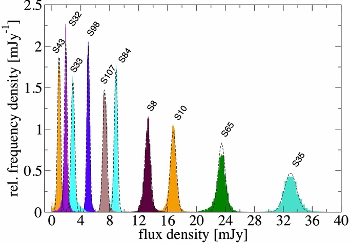
Footnotes
- 6
∼20 minutes at the innermost stable orbit for Sgr A*.
- 7
- 8
And accordingly with different pixel samplings of 13 mas pixel−1 and 27 mas pixel−1.
- 9
This is a method to reject frames of lower quality with respect to the majority of the individual observation night. For each sub-frame of the night (i.e., the part of the jittered frames that is common to all) we count the stars detected by Starfinder. We then calculate the average number of detections over the night and the standard deviation and reject all frames with a negative deviation from the average of more than 1.7 times the standard deviation.
- 10
Which is the reason why Dodds-Eden et al. (2011) did not include the 2003 data which is clearly visible in the 2004 epoch of their uncorrected light curve.
- 11
Slightly shifted on the x-axis to account for the proper offset due to the double aperture method used by Dodds-Eden et al. (2011), which we included only roughly by adding 3 mJy, and to make it best fit the extremes of our histogram.
- 12
The latter we show in an unweighted version and in an integration time-weighted version.
- 13
This of course corresponds to a hyperbolic increase of the relative error toward small flux densities.
- 14
Because the shape of the intrinsic distribution close to the detection limit cannot be determined accurately enough to make a difference between a log-normal behavior and a truncated power law.
- 15
The latter allows for a separation of the part of the histogram that is assumed to represent the intrinsic distribution of flux densities (>xmin) from the part dominated by instrumental effects.
- 16
i.e., light curves with a time correlation characterized by a power-law-like power spectral density