Visualizing Gradients

Author: Justin Silver

This tutorial explains the subtleties of requires_grad, retain_grad, leaf, and non-leaf tensors using a simple example. It then covers how to extract and visualize gradients at any layer in a neural network. By inspecting how information flows from the end of the network to the parameters we want to optimize, we can debug issues such as vanishing or exploding gradients that occur during training.

Before starting, make sure you understand tensors and how to manipulate them. A basic knowledge of how autograd works would also be useful.

Setup

First, make sure PyTorch is installed and then import the necessary libraries.

import torch
import torch.nn as nn
import torch.optim as optim
import torch.nn.functional as F
import matplotlib.pyplot as plt

Next, we instantiate a simple network to focus on the gradients. This will be an affine layer, followed by a ReLU activation, and ending with a MSE loss between prediction and label tensors.

\[\mathbf{y}_{\text{pred}} = \text{ReLU}(\mathbf{x} \mathbf{W} + \mathbf{b})\]

\[L = \text{MSE}(\mathbf{y}_{\text{pred}}, \mathbf{y})\]

Note that the requires_grad=True is necessary for the parameters (W and b) so that PyTorch tracks operations involving those tensors. We’ll discuss more about this in a future section.

# tensor setup
x = torch.ones(1, 3)                      # input with shape: (1, 3)
W = torch.ones(3, 2, requires_grad=True)  # weights with shape: (3, 2)
b = torch.ones(1, 2, requires_grad=True)  # bias with shape: (1, 2)
y = torch.ones(1, 2)                      # output with shape: (1, 2)

# forward pass
z = (x @ W) + b                           # pre-activation with shape: (1, 2)
y_pred = F.relu(z)                        # activation with shape: (1, 2)
loss = F.mse_loss(y_pred, y)              # scalar loss

Leaf vs. non-leaf tensors

After running the forward pass, PyTorch autograd has built up a dynamic computational graph which is shown below. This is a Directed Acyclic Graph (DAG) which keeps a record of input tensors (leaf nodes), all subsequent operations on those tensors, and the intermediate/output tensors (non-leaf nodes). The graph is used to compute gradients for each tensor starting from the graph roots (outputs) to the leaves (inputs) using the chain rule from calculus:

\[\mathbf{y} = \mathbf{f}_k\bigl(\mathbf{f}_{k-1}(\dots \mathbf{f}_1(\mathbf{x}) \dots)\bigr)\]

\[\frac{\partial \mathbf{y}}{\partial \mathbf{x}} = \frac{\partial \mathbf{f}_k}{\partial \mathbf{f}_{k-1}} \cdot \frac{\partial \mathbf{f}_{k-1}}{\partial \mathbf{f}_{k-2}} \cdot \cdots \cdot \frac{\partial \mathbf{f}_1}{\partial \mathbf{x}}\]

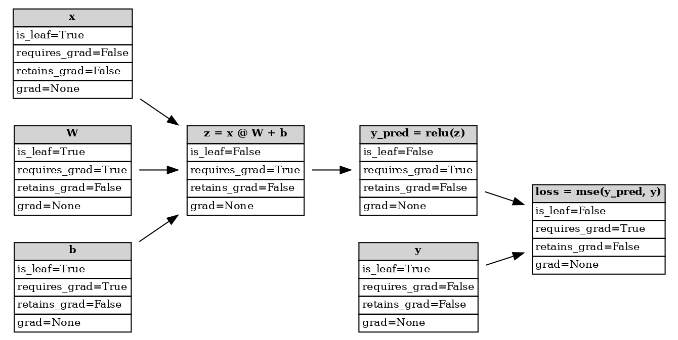
Computational graph after forward pass

PyTorch considers a node to be a leaf if it is not the result of a tensor operation with at least one input having requires_grad=True (e.g. x, W, b, and y), and everything else to be non-leaf (e.g. z, y_pred, and loss). You can verify this programmatically by probing the is_leaf attribute of the tensors:

# prints True because new tensors are leafs by convention
print(f"{x.is_leaf=}")

# prints False because tensor is the result of an operation with at
# least one input having requires_grad=True
print(f"{z.is_leaf=}")

x.is_leaf=True
z.is_leaf=False

The distinction between leaf and non-leaf determines whether the tensor’s gradient will be stored in the grad property after the backward pass, and thus be usable for gradient descent. We’ll cover this some more in the following section.

Let’s now investigate how PyTorch calculates and stores gradients for the tensors in its computational graph.

requires_grad

To build the computational graph which can be used for gradient calculation, we need to pass in the requires_grad=True parameter to a tensor constructor. By default, the value is False, and thus PyTorch does not track gradients on any created tensors. To verify this, try not setting requires_grad, re-run the forward pass, and then run backpropagation. You will see:

>>> loss.backward()
RuntimeError: element 0 of tensors does not require grad and does not have a grad_fn

This error means that autograd can’t backpropagate to any leaf tensors because loss is not tracking gradients. If you need to change the property, you can call requires_grad_() on the tensor (notice the _ suffix).

We can sanity check which nodes require gradient calculation, just like we did above with the is_leaf attribute:

print(f"{x.requires_grad=}") # prints False because requires_grad=False by default
print(f"{W.requires_grad=}") # prints True because we set requires_grad=True in constructor
print(f"{z.requires_grad=}") # prints True because tensor is a non-leaf node

x.requires_grad=False
W.requires_grad=True
z.requires_grad=True

It’s useful to remember that a non-leaf tensor has requires_grad=True by definition, since backpropagation would fail otherwise. If the tensor is a leaf, then it will only have requires_grad=True if it was specifically set by the user. Another way to phrase this is that if at least one of the inputs to a tensor requires the gradient, then it will require the gradient as well.

There are two exceptions to this rule:

1. Any nn.Module that has nn.Parameter will have requires_grad=True for its parameters (see here)

2. Locally disabling gradient computation with context managers (see here)

In summary, requires_grad tells autograd which tensors need to have their gradients calculated for backpropagation to work. This is different from which tensors have their grad field populated, which is the topic of the next section.

retain_grad

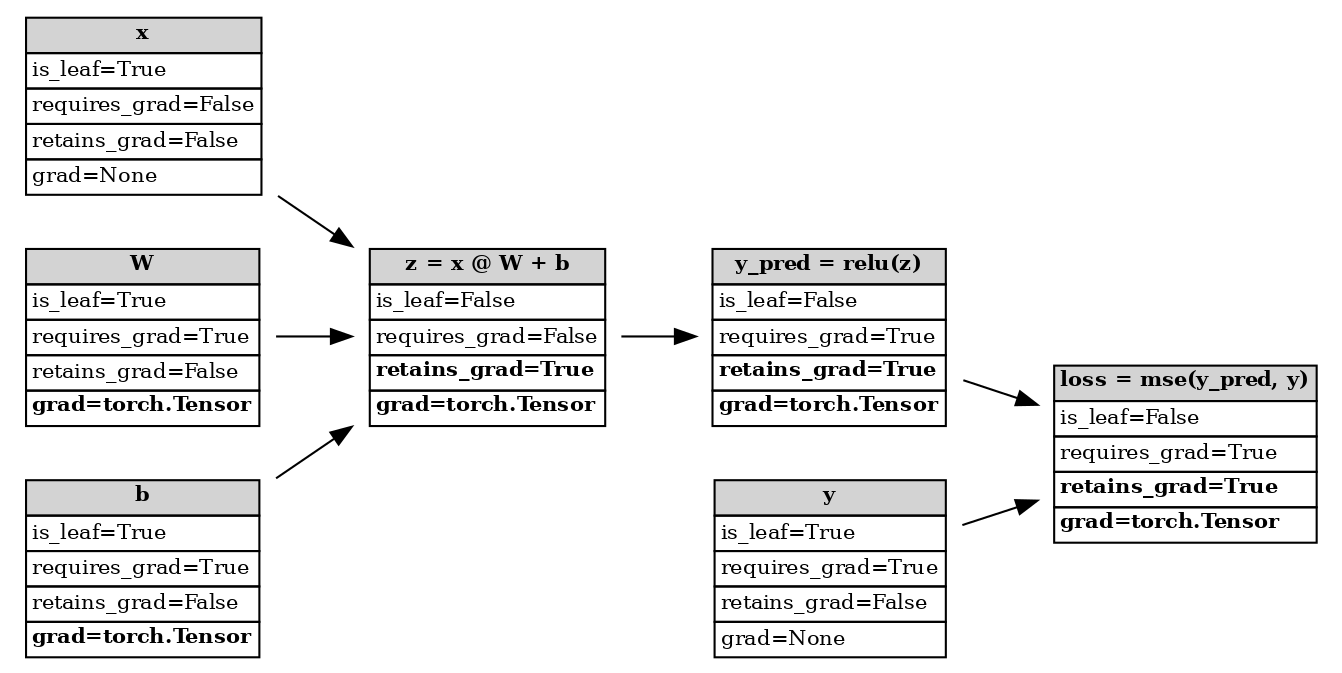
To actually perform optimization (e.g. SGD, Adam, etc.), we need to run the backward pass so that we can extract the gradients.

loss.backward()

Calling backward() populates the grad field of all leaf tensors which had requires_grad=True. The grad is the gradient of the loss with respect to the tensor we are probing. Before running backward(), this attribute is set to None.

print(f"{W.grad=}")
print(f"{b.grad=}")

W.grad=tensor([[3., 3.],
        [3., 3.],
        [3., 3.]])
b.grad=tensor([[3., 3.]])

You might be wondering about the other tensors in our network. Let’s check the remaining leaf nodes:

# prints all None because requires_grad=False
print(f"{x.grad=}")
print(f"{y.grad=}")

x.grad=None
y.grad=None

The gradients for these tensors haven’t been populated because we did not explicitly tell PyTorch to calculate their gradient (requires_grad=False).

Let’s now look at an intermediate non-leaf node:

print(f"{z.grad=}")

/var/lib/workspace/advanced_source/visualizing_gradients_tutorial.py:227: UserWarning:

The .grad attribute of a Tensor that is not a leaf Tensor is being accessed. Its .grad attribute won't be populated during autograd.backward(). If you indeed want the .grad field to be populated for a non-leaf Tensor, use .retain_grad() on the non-leaf Tensor. If you access the non-leaf Tensor by mistake, make sure you access the leaf Tensor instead. See github.com/pytorch/pytorch/pull/30531 for more informations. (Triggered internally at /pytorch/build/aten/src/ATen/core/TensorBody.h:489.)

z.grad=None

PyTorch returns None for the gradient and also warns us that a non-leaf node’s grad attribute is being accessed. Although autograd has to calculate intermediate gradients for backpropagation to work, it assumes you don’t need to access the values afterwards. To change this behavior, we can use the retain_grad() function on a tensor. This tells the autograd engine to populate that tensor’s grad after calling backward().

# we have to re-run the forward pass
z = (x @ W) + b
y_pred = F.relu(z)
loss = F.mse_loss(y_pred, y)

# tell PyTorch to store the gradients after backward()
z.retain_grad()
y_pred.retain_grad()
loss.retain_grad()

# have to zero out gradients otherwise they would accumulate
W.grad = None
b.grad = None

# backpropagation
loss.backward()

# print gradients for all tensors that have requires_grad=True
print(f"{W.grad=}")
print(f"{b.grad=}")
print(f"{z.grad=}")
print(f"{y_pred.grad=}")
print(f"{loss.grad=}")

W.grad=tensor([[3., 3.],
        [3., 3.],
        [3., 3.]])
b.grad=tensor([[3., 3.]])
z.grad=tensor([[3., 3.]])
y_pred.grad=tensor([[3., 3.]])
loss.grad=tensor(1.)

We get the same result for W.grad as before. Also note that because the loss is scalar, the gradient of the loss with respect to itself is simply 1.0.

If we look at the state of the computational graph now, we see that the retains_grad attribute has changed for the intermediate tensors. By convention, this attribute will print False for any leaf node, even if it requires its gradient.

Computational graph after backward pass

If you call retain_grad() on a non-leaf node, it results in a no-op. If we call retain_grad() on a node that has requires_grad=False, PyTorch actually throws an error, since it can’t store the gradient if it is never calculated.

>>> x.retain_grad()
RuntimeError: can't retain_grad on Tensor that has requires_grad=False

Summary table

Using retain_grad() and retains_grad only make sense for non-leaf nodes, since the grad attribute will already be populated for leaf tensors that have requires_grad=True. By default, these non-leaf nodes do not retain (store) their gradient after backpropagation. We can change that by rerunning the forward pass, telling PyTorch to store the gradients, and then performing backpropagation.

The following table can be used as a reference which summarizes the above discussions. The following scenarios are the only ones that are valid for PyTorch tensors.

is_leaf	requires_grad	retains_grad	require_grad()	retain_grad()
True	False	False	sets requires_grad to True or False	no-op
True	True	False	sets requires_grad to True or False	no-op
False	True	False	no-op	sets retains_grad to True
False	True	True	no-op	no-op

Real world example with BatchNorm

Let’s move on from the toy example above and study a more realistic network. We’ll be creating a network intended for the MNIST dataset, similar to the architecture described by the batch normalization paper.

To illustrate the importance of gradient visualization, we will instantiate one version of the network with batch normalization (BatchNorm), and one without it. Batch normalization is an extremely effective technique to resolve vanishing/exploding gradients, and we will be verifying that experimentally.

The model we use has a configurable number of repeating fully-connected layers which alternate between nn.Linear, norm_layer, and nn.Sigmoid. If batch normalization is enabled, then norm_layer will use BatchNorm1d, otherwise it will use the Identity transformation.

def fc_layer(in_size, out_size, norm_layer):
    """Return a stack of linear->norm->sigmoid layers"""
    return nn.Sequential(nn.Linear(in_size, out_size), norm_layer(out_size), nn.Sigmoid())

class Net(nn.Module):
    """Define a network that has num_layers of linear->norm->sigmoid transformations"""
    def __init__(self, in_size=28*28, hidden_size=128,
                 out_size=10, num_layers=3, batchnorm=False):
        super().__init__()
        if batchnorm is False:
            norm_layer = nn.Identity
        else:
            norm_layer = nn.BatchNorm1d

        layers = []
        layers.append(fc_layer(in_size, hidden_size, norm_layer))

        for i in range(num_layers-1):
            layers.append(fc_layer(hidden_size, hidden_size, norm_layer))

        layers.append(nn.Linear(hidden_size, out_size))

        self.layers = nn.Sequential(*layers)

    def forward(self, x):
        x = torch.flatten(x, 1)
        return self.layers(x)

Next we set up some dummy data, instantiate two versions of the model, and initialize the optimizers.

# set up dummy data
x = torch.randn(10, 28, 28)
y = torch.randint(10, (10, ))

# init model
model_bn = Net(batchnorm=True, num_layers=3)
model_nobn = Net(batchnorm=False, num_layers=3)

model_bn.train()
model_nobn.train()

optimizer_bn = optim.SGD(model_bn.parameters(), lr=0.01, momentum=0.9)
optimizer_nobn = optim.SGD(model_nobn.parameters(), lr=0.01, momentum=0.9)

We can verify that batch normalization is only being applied to one of the models by probing one of the internal layers:

print(model_bn.layers[0])
print(model_nobn.layers[0])

Sequential(
  (0): Linear(in_features=784, out_features=128, bias=True)
  (1): BatchNorm1d(128, eps=1e-05, momentum=0.1, affine=True, track_running_stats=True)
  (2): Sigmoid()
)
Sequential(
  (0): Linear(in_features=784, out_features=128, bias=True)
  (1): Identity()
  (2): Sigmoid()
)

Because we wrapped up the logic and state of our model in a nn.Module, we need another method to access the intermediate gradients if we want to avoid modifying the module code directly. This is done by registering a hook.

Warning

Using backward pass hooks attached to output tensors is preferred over using retain_grad() on the tensors themselves. An alternative method is to directly attach module hooks (e.g. register_full_backward_hook()) so long as the nn.Module instance does not do perform any in-place operations. For more information, please refer to this issue.

The following code defines our hooks and gathers descriptive names for the network’s layers.

# note that wrapper functions are used for Python closure
# so that we can pass arguments.

def hook_forward_wrapper(module_name, grads):
    def hook_forward(module, args, output):
        """Forward pass hook which attaches backward pass hooks to intermediate tensors"""
        output.register_hook(hook_backward_wrapper(module_name, grads))
    return hook_forward

def hook_backward_wrapper(module_name, grads):
    def hook_backward(grad):
        """Backward pass hook which appends gradients"""
        grads.append((module_name, grad))
    return hook_backward

def get_all_layers(model, hook_fn):
    """Register forward pass hook (hook_fn) to model outputs

    Returns:
        - layers: a dict with keys as layer/module and values as layer/module names
                  e.g. layers[nn.Conv2d] = layer1.0.conv1
        - grads: a list of tuples with module name and tensor output gradient
                 e.g. grads[0] == (layer1.0.conv1, tensor.Torch(...))
    """
    layers = dict()
    grads = []
    for name, layer in model.named_modules():
        # skip Sequential and/or wrapper modules
        if any(layer.children()) is False:
            layers[layer] = name
            layer.register_forward_hook(hook_fn(name, grads))
    return layers, grads

# register hooks
layers_bn, grads_bn = get_all_layers(model_bn, hook_forward_wrapper)
layers_nobn, grads_nobn = get_all_layers(model_nobn, hook_forward_wrapper)

Let’s now train the models for a few epochs:

epochs = 10

for epoch in range(epochs):

    # important to clear, because we append to
    # outputs everytime we do a forward pass
    grads_bn.clear()
    grads_nobn.clear()

    optimizer_bn.zero_grad()
    optimizer_nobn.zero_grad()

    y_pred_bn = model_bn(x)
    y_pred_nobn = model_nobn(x)

    loss_bn = F.cross_entropy(y_pred_bn, y)
    loss_nobn = F.cross_entropy(y_pred_nobn, y)

    loss_bn.backward()
    loss_nobn.backward()

    optimizer_bn.step()
    optimizer_nobn.step()

After running the forward and backward pass, the gradients for all the intermediate tensors should be present in grads_bn and grads_nobn. We compute the mean absolute value of each gradient matrix so that we can compare the two models.

def get_grads(grads):
    layer_idx = []
    avg_grads = []
    for idx, (name, grad) in enumerate(grads):
        if grad is not None:
            avg_grad = grad.abs().mean()
            avg_grads.append(avg_grad)
            # idx is backwards since we appended in backward pass
            layer_idx.append(len(grads) - 1 - idx)
    return layer_idx, avg_grads

layer_idx_bn, avg_grads_bn = get_grads(grads_bn)
layer_idx_nobn, avg_grads_nobn = get_grads(grads_nobn)

With the average gradients computed, we can now plot them and see how the values change as a function of the network depth. Notice that when we don’t apply batch normalization, the gradient values in the intermediate layers fall to zero very quickly. The batch normalization model, however, maintains non-zero gradients in its intermediate layers.

fig, ax = plt.subplots()
ax.plot(layer_idx_bn, avg_grads_bn, label="With BatchNorm", marker="o")
ax.plot(layer_idx_nobn, avg_grads_nobn, label="Without BatchNorm", marker="x")
ax.set_xlabel("Layer depth")
ax.set_ylabel("Average gradient")
ax.set_title("Gradient flow")
ax.grid(True)
ax.legend()
plt.show()

Conclusion

In this tutorial, we covered when and how PyTorch computes gradients for leaf and non-leaf tensors. By using retain_grad, we can access the gradients of intermediate tensors within autograd’s computational graph. Building upon this, we then demonstrated how to visualize the gradient flow through a neural network wrapped in a nn.Module class. We qualitatively showed how batch normalization helps to alleviate the vanishing gradient issue which occurs with deep neural networks.

If you would like to learn more about how PyTorch’s autograd system works, please visit the references below. If you have any feedback for this tutorial (improvements, typo fixes, etc.) then please use the PyTorch Forums and/or the issue tracker to reach out.

(Optional) Additional exercises

• Try increasing the number of layers (num_layers) in our model and see what effect this has on the gradient flow graph

• How would you adapt the code to visualize average activations instead of average gradients? (Hint: in the hook_forward() function we have access to the raw tensor output)

• What are some other methods to deal with vanishing and exploding gradients?

References

• A Gentle Introduction to torch.autograd

• Automatic Differentiation with torch.autograd

• Autograd mechanics

• Batch Normalization: Accelerating Deep Network Training by Reducing Internal Covariate Shift

• On the difficulty of training Recurrent Neural Networks