


Abstract
We construct a physically parameterized probabilistic autoencoder (PAE) to learn the intrinsic diversity of Type Ia supernovae (SNe Ia) from a sparse set of spectral time series. The PAE is a two-stage generative model, composed of an autoencoder that is interpreted probabilistically after training using a normalizing flow. We demonstrate that the PAE learns a low-dimensional latent space that captures the nonlinear range of features that exists within the population and can accurately model the spectral evolution of SNe Ia across the full range of wavelength and observation times directly from the data. By introducing a correlation penalty term and multistage training setup alongside our physically parameterized network, we show that intrinsic and extrinsic modes of variability can be separated during training, removing the need for the additional models to perform magnitude standardization. We then use our PAE in a number of downstream tasks on SNe Ia for increasingly precise cosmological analyses, including the automatic detection of SN outliers, the generation of samples consistent with the data distribution, and solving the inverse problem in the presence of noisy and incomplete data to constrain cosmological distance measurements. We find that the optimal number of intrinsic model parameters appears to be three, in line with previous studies, and show that we can standardize our test sample of SNe Ia with an rms of 0.091 ± 0.010 mag, which corresponds to 0.074 ± 0.010 mag if peculiar velocity contributions are removed. Trained models and codes are released at https://github.com/georgestein/suPAErnova.
Export citation and abstract BibTeX RIS

Original content from this work may be used under the terms of the Creative Commons Attribution 4.0 licence. Any further distribution of this work must maintain attribution to the author(s) and the title of the work, journal citation and DOI.
1. Introduction
Type Ia supernovae (SNe Ia) are excellent probes of cosmic history, leading to the discovery of the accelerating expansion of the universe (Riess et al. 1998; Perlmutter et al. 1999). Their cosmological utility emerges from the high degree of similarity between each SN Ia, and differences in their luminosity have been shown to strongly correlate with observed spectro-temporal features. As such, they can be used as "standardizable candles" to infer the relative distances to them through a measurement of their fluxes, which alongside a measurement of their redshift allows for the expansion history of the universe to be inferred (Riess et al. 1998; Perlmutter et al. 1999; Betoule et al. 2014; Scolnic et al. 2018).
The limiting factor in using SNe Ia for increasingly precise cosmological analyses is a detailed understanding of their spectral diversity and evolution, which cannot be modeled from first principles to high enough accuracy. Thus, the field relies on data-driven models, which have uncovered a number of well-known relations between SN Ia features and luminosity, including the correlation between the peak luminosity of an SN Ia and the light-curve decrease time (brighter-slower effect; Phillips 1993) and the dependence of the peak luminosity on color (the brighter-bluer effect Riess et al. 1996; Tripp 1998). These behaviors are captured in conventional light-curve-fitting routines such as SALT2 (Guy et al. 2007), MLCS2k2 (Jha et al.2007), and SNooPy (Burns et al. 2011), and their associated standardization parameters.
While these effects correlate with a high degree of spectral variation, they are insufficient to fully account for the detailed differences between spectral and temporal features of different SNe Ia. To try to understand spectral behavior in more detail, collections of SN Ia spectra (e.g., Matheson et al. 2008; Bailey et al. 2009; Silverman et al. 2012b; Folatelli et al. 2013; Stahl et al. 2020b) have been used to examine the strengths, ratios, and velocities of specific spectral features (e.g., Nugent et al. 1995; Folatelli 2004; Folatelli et al. 2010, 2013; Branch et al. 2006; Arsenijevic et al. 2008; Bailey et al. 2009; Foley et al. 2011; Silverman et al. 2012a; Blondin et al. 2012; Wang et al. 2013) and correlate these with SN Ia brightness, color, and decline rate.
With the advent of full SN Ia spectral time series (Aldering et al. 2020) or their virtually constructed analogs (Siebert et al. 2019; Stahl et al. 2020b), it has become possible to study the full spectro-temporal behavior of SNe Ia. Examples include the first construction of a spectral metric space (Sasdelli et al. 2015), Gaussian Process (GP) twinning (Fakhouri et al. 2015), expectation maximization factor analysis (Saunders et al. 2018), spectral feature factor analysis (Léget et al. 2020), an SN Ia autoencoder (Sasdelli et al. 2016) hierarchical Bayesian spectro-temporal modeling (Mandel et al. 2022), deep learning (Stahl et al. 2020a), and the nonlinear Twins Embedding space of Boone et al. (2021a, 2021b).
Such models must be able to account for both extrinsic and intrinsic modes of spectral diversity. Intrinsic effects result from object-to-object differences between SN explosions, while extrinsic effects are differences caused by physical processes external to the SN system. Examples of extrinsic effects include the amount of Galactic and extragalactic dust along the sight line to the object (and hence extinction), and the peculiar velocity of the SN with respect to our observational rest frame, which should therefore be uncorrelated with the intrinsic properties of the SN Ia. Depending on the specific empirical model, they can be used for applications including magnitude standardization, anomaly detection, and uncertainty estimates.
1.1. Empirical Modeling of SNe Ia
After the initial explosion, an SN continues to brighten until it reaches a peak and begins to fade, with the observable lifecycle (for the purpose of this work) taking on the order of ∼50 days. Accurately modeling this SN luminosity as a function of time is challenging due to both the small number of spectroscopically observed SNe Ia and the highly irregular time sampling of spectra from each object, where for most SNe we observe only ∼10 spectra spread over the range. This sparse time sampling can prove difficult for numerical techniques that require more uniform observations, so fitting an empirical model of SN flux as a function of time and wavelength often has two steps. The first is to interpolate the observations from each SN onto a more regularly spaced time grid, generally achieved through spline interpolations or Gaussian processes. The second is to then model the spectrum at each temporal location and wavelength bin on this time grid. The most commonly used models are based on variations of a principal component analysis (PCA) and schematically take a form that separates intrinsic and extrinsic physical effects into unique terms:

where p is the time from peak brightness and λ is the rest-frame wavelength. The average spectral sequence is described by F0(t, λ), the components that describe additional PCA variability are Fn
(t, λ), where n > 0, and the color term representing both extinction and intrinsic color variations of the global model. The parameters indicated with an  subscript are fit to each SN and correspond to PCA amplitudes
  and the extinction
  . The terms of the model are split this way for a few key reasons:
Amplitude: For each SN, the observed redshift zobs is generally well known, such that the wavelength and timescales can be accurately de-redshifted. The observed redshift has contributions from the peculiar velocity of the SN, which are extrinsic to the SN explosion. A leading amplitude term then ensures that the peculiar velocity component is not correlated with the model parameters and that it is the only coefficient dependent on the flux normalization. This amplitude can interchangeably be written as 10−0.4ΔM when working in magnitudes.
Color law: The color law attempts to account for dust along the line of sight to the SNe. The optical depth to each SN involves a number of factors, including corrections from the local environment of the SNe and its host galaxy, and line-of-sight variations along the intergalactic medium and within our own galaxy. The Milky Way extinction can be determined independently and removed from the observed spectrum. Any optical depth variations along the line of sight should be slowly varying with respect to the ∼50 day observation window of an SN (Huang et al. 2017), and therefore should be dependent only on the wavelength of observation. This color law is generally an input to the model (Guy et al. 2007; Saunders et al.2018; Mandel et al. 2022; Boone et al. 2021a), and any time-dependent color variation should be captured by the variations in the global model.
To use such an empirical model for magnitude standardization then requires an additional third step, in which the (possible) correlations between model parameters and intrinsic luminosity are uncovered. This requires an additional model to be fit to "explain" the magnitude residual as a function of the model parameters from previous steps.
In this work, we propose an alternative to this three-step workflow—a probabilistic autoencoder (PAE) to model SNe spectra as a function of observation time. As introduced by Böhm & Seljak (2020), a PAE combines the advantages of an autoencoder (i.e., it is fast and easy to train) with the desired properties of a generative model, which makes a PAE a powerful tool for probabilistic data reconstruction and outlier detection of SNe Ia. We physically parameterize our PAE and introduce a multistage training setup and correlation penalty term in order to separate and decorrelate intrinsic and extrinsic effects during training, which removes the need for an additional model to perform magnitude standardization.
Our method has a number of advantages over PCA-based models. First, the autoencoder has the ability to learn complicated nonlinear mappings between the best-fit latent representations (parameters), while a PCA analysis is limited to linear transformations. This allows for increased spectral diversity to be expressed over linear models for a given latent dimensionality. Second, the probabilistic nature of the PAE allows for a straightforward determination of outlying spectra and calculation of the errors on the best-fit model parameters within the observational errors. A conditional autoencoder (AE) can account for time-evolution by simply feeding in the observation times as a conditional parameter, and does not need to first pre-process the data to interpolate it onto a regular grid, which allows the model to work directly on the data. Finally, a PAE model can be used to generate artificial SNe Ia samples consistent with the data distribution, and to create a faithful simulation of SNe Ia spectro-temporal series.
The outline of this paper is as follows. We first describe the data set and reference baselines in Section 2, followed by a detailed description of probabilistic autoencoders in Section 3. We then outline our architecture and training setup in Section 4. Section 5 showcases the PAE results, where we demonstrate that the PAE provides better fits to the observations than the most commonly used model in the literature, it automatically detects outliers, and provides an accurate fit on SNe parameters and their errors. A discussion follows in Section 6.
2. Data Set and Reference Baselines
Our data set consists of spectral time series data of 228 unique SNe Ia, obtained by the Nearby Supernova Factory (SNfactory; Aldering et al. 2002, 2020) using the SuperNova Integral Field Spectrograph (SNIFS; Lantz et al. 2004). The original spectra span the range 3200–10000 Å simultaneously. The spectra from SNIFS were reduced using the SNfactory data reduction pipeline (Bacon et al. 2001; Aldering et al. 2006; Scalzo et al. 2010), flux calibrated following Buton et al. (2013), Rubin et al. (2022), and host-galaxy subtracted as in Bongard et al. (2011). The spectra were corrected for dust in our Galaxy using the dust map from Schlegel et al. (1998) and the extinction–color relation from Cardelli et al. (1989).
Following our past procedure for similar analyses (Fakhouri et al. 2015; Saunders et al. 2018; Aldering et al. 2020; Léget et al. 2020; Boone et al. 2021a, 2021b), the wavelength and phases have been transformed to the rest frame, and the fluxes have been transformed to a reference redshift of z = 0.05 using the appropriate factors of z and 1 + z using redshifts from Childress et al. (2013) and Rigault et al. (2020). Because SN Ia spectral features are broad, the spectra are rebinned to a common rest-frame wavelength binning of 1000 km s−1 between 3300 and 8600 Å, resulting in Nλ
= 288 rest frame wavelength bins. Each spectrum is accompanied by an uncertainty spectrum,  . A small number of spectra do not cover all wavelength bins, therefore, for each spectrum, we construct a mask array
  to flag any missing wavelength bins.
Each SN has between 5 and 64 observations at different times, for a total of 3034 spectra. The time gaps between each observation are typically in the range of 2–3 days at early phases and longer at later phases, but with exceptions due to, e.g., bad weather. The given observation time p is the phase relative to the peak luminosity of the SNe in the B band as fit by the SALT2 model (Guy et al. 2007), in days. The SALT2 fits also report an uncertainty on the time on peak luminosity. We cut data outside of (−10 days, +40 days), resulting in 2696 final spectra for a minimum of 4 observations of an SN, to a maximum of 32. The amplitudes of the spectra, initially in the z = 0.05 reference frame, are multiplied by a constant to scale the range of values to ∼(0,1).
At a given observation time, spectra from different SNe have a high degree of similarity, and it is easy to imagine each unique spectra being described by a set of modifications to some mean spectral envelope as a function of time. It has been shown before that the leading few components in a PCA analysis capture a significant amount of the SN-to-SN variation (Guy et al. 2007; Saunders et al. 2018), so we expect the data to be able to be represented by an autoencoder with some small set of latent variables.
2.1. Reference Baselines
Throughout this work we compare our spectral reconstructions to the SALT2 model (Guy et al. 2007), and compare our cosmological distance measurements to both the SALT2 model and the Twins Embedding (Boone et al. 2021a, 2021b).
2.1.1. SALT2
SALT2 (Guy et al. 2007) models the time-evolving spectral energy distribution as

where p is the rest-frame time since the date of maximum luminosity in the B band and λ is the rest-frame wavelength. The M0 component is the average spectral sequence, Mi
for i > 0 are additional components that describe further object-to-object variability, and CL(λ) is a generic color term that mixes dust extinction and intrinsic color variations left over after decorrelating x1 and c. Each individual SN is then parameterized by a combination of these components multiplied by leading amplitude terms describing the strength of each:  , and cSN.
  is the flux normalization and is a function of both the intrinsic luminosity and the luminosity distance of the SN. The best-fit SALT2 parameters
  ,
,  , and cSN were fit for each light curve in the data set, and we used sncosmo (Barbary et al. 2016) to generate the best-fit rest frame SALT2 spectra for each SN at each observation time.
The SALT2 light-curve fits are used to determine the peak brightness of each SN Ia, and then a linear correction for the light-curve width and color is applied to "explain" the magnitude residual to each object as a function of the other model parameters:

The arbitrary reference magnitude Mref and standardization parameters α and β are fit in order to minimize the magnitude residual  .
.
2.1.2. Twins Embedding
The Twins Embedding (Boone et al. 2021a, 2021b) does not model temporal evolution and instead aims to explain the spectral variability of SNe Ia at maximum light. There are four separate components to the model:
- 1.A differential time-evolution model to estimate a spectrum at maximum light for each SN Ia.
- 2.A second "Reading Between the Lines" (RBTL) model to fit for a mean spectrum at maximum light, fmean(λ), and explain the SN-to-SN variability at maximum light as a function of two parameters ΔMi and ΔAV,i ,ΔMi is the difference in intrinsic brightness compared to the mean spectrum in magnitudes, and ΔAV,i represents the coefficient of the extinction–color relation that best matches the SN's spectrum to the mean function. The RBTL model is used to deredden each spectrum at maximum light to remove extrinsic contributions from distance uncertainties and interstellar dust.

- 3.A third nonlinear "Twins Embedding" model is trained on the dereddened spectra from the RBTL model in order to further explain any variability of SN Ia spectra at maximum light. The Twins Embedding uses the Isomap algorithm (Tenenbaum et al. 2000) to embed the spectral distancebetween two SNe Ia labeled i and j into a low-dimensional (3D) space ξ while preserving the distances between nearby points in the high-dimensional space.
- 4.GP regression is then used to infer the magnitude residuals (ΔMi from step 2) of SNe Ia over the 3D Twins Embedding space ξ and to reconstruct spectra from a given embedding vector. The inferred value of the magnitude residual can be subtracted from the measured value, and the remainder represents the "unexplained residual."


Dixon et al. (in preparation) extend this Twins Embedding to the full time series using a neural network.
3. Physically Parameterized Probabilistic Autoencoder
Our probabilistic autoencoder is constructed in two separate stages. First, we train a conditional autoencoder to learn a low-dimensional latent representation of each SN that is independent of the observation time(s). After the autoencoder is trained we construct a normalizing flow to map from the unconstrained autoencoder latent space to a Gaussian latent space. For clarity, our data notation is as follows, where for each SN, arrays are filled sequentially using the observed spectra:
- 1.: observed SNe Ia spectral time series.
- 2.: reconstructed SNe Ia spectral time series.
- 3.: observational uncertainty.
- 4.: observational mask, equal to 1 where spectra are valid.
- 5.: observation time of each spectrum relative to the peak brightness of the SNe.
- 6.: Autoencoder latent space (Δp, ΔM, ΔAV
, z1,...,zn
).
- (a)Δp: Difference in time of peak brightness relative to the SALT2 fits (any float value).
- (b)ΔM: magnitude residual.
- (c)ΔAV : relative extrinsic extinction.
- 7.: normalizing flow latent space. Nlatent−2 results from the removal of Δp and ΔM.


For purely practical purposes, when the number of observations of an SN is less than the maximum in the data set, Nobs = 32, the end of the data arrays are zero-padded and masked appropriately to fill any remaining empty observation vectors. This has no effect on the model beyond simplifying the training procedure.
3.1. Conditional Autoencoder
An autoencoder consists of an encoder that maps the input data to a lower-dimensional latent representation and a decoder that reconstructs the data from the latent representation. Both of these components are commonly parameterized as deep neural networks, with weights and biases trained through back-propagation to minimize a loss function. Autoencoders are commonly used for dimensionality reduction or feature learning from an arbitrary dimensional data space, but here we introduce a number of modifications from a general architecture to describe the physical nature of the data set and separate external and internal information of the SNe.
The encoder f maps the spectral time series to a latent space (Δp, ΔM, ΔAV , z ) = f ( x , p ) through a series of fully connected layers of a neural network. Operations are performed along the wavelength axis only, and each spectrum from an SN is treated independently until the final network layer. The final layer reduces to the mean latent representation of an SN along the time axis for all observations of the SN Ia, such that the coordinates of each SN are forced to represent a compression of the SN as an object and not a compression of each individual spectra. In this way, the entire spectral time series of a SN is reduced to a few latent variables that together represent a nonlinear combination of components describing object-to-object variability, such as the luminosity, spectral tilt, or absorption lines.
Given a latent representation and observation times the decoder
g
learns to reconstruct the spectral time series  . The decoder first duplicates and concatenates the latent representation
z
with the observation phases
p
, then passes this through a number of fully connected layers. Again, the latent and time-variable concatenation operations are performed along the wavelength axis only, and each spectrum from an SN is treated independently. We parameterize the decoder similar to Equation (2) by not passing some latent parameters through the fully connected layers of the decoder, and instead separating them out to represent an overall amplitude and a phase-independent color law term, which are multiplied with the output of the final layer. The encoder and decoder are both fully connected deep neural networks, trained to maximize the agreement of the reconstruction with the data, determined through a loss function
. The decoder first duplicates and concatenates the latent representation
z
with the observation phases
p
, then passes this through a number of fully connected layers. Again, the latent and time-variable concatenation operations are performed along the wavelength axis only, and each spectrum from an SN is treated independently. We parameterize the decoder similar to Equation (2) by not passing some latent parameters through the fully connected layers of the decoder, and instead separating them out to represent an overall amplitude and a phase-independent color law term, which are multiplied with the output of the final layer. The encoder and decoder are both fully connected deep neural networks, trained to maximize the agreement of the reconstruction with the data, determined through a loss function  .
.
While separating out certain latent parameters to represent physical variables is uncommon in autoencoder literature, it is desirable here due to the physical nature of the problem we are attempting to solve. The time-independent color law term is separated out as we expect that a portion of the color is from the reddening of the spectrum as it propagates through dust in the intragalactic medium. This effect is independent of the intrinsic SN Ia explosion and so should not propagate through to all the latent variables of the model. The amplitude is separated out as a number of physical effects unrelated to the true cosmological distance can shift the spectra in a way uncorrelated with any spectral features. Peculiar velocity contributions to the redshifts result in an amplitude shift of less than ∼10% for higher-redshift SNe (z > 0.02). Additionally, the spectra have instrumental "gray" offsets of a few percent (e.g., Rubin et al. 2022) that also look like an amplitude. These are unique to each spectrum individually and are typically around ∼2%, but the distribution is very non-Gaussian. Without allowing for an explicit amplitude term in the model, any amplitude that is by definition uncorrelated with the spectral features will propagate through to uncertainty in the inferred cosmological distance. Our model thus takes the form of

where CL(λ) can be fit during training by using a single dense layer or can be adopted from physical measurements (e.g., Fitzpatrick 1999; we set RV = 2.8). We refer to both the 10−0.4ΔM component and the ΔM parameter as the extrinsic amplitude of the model throughout this work, but we note that an extrinsic interpretation of ΔM is degenerate with an intrinsic component that does not vary with wavelength or phase.
We have found that separating out the amplitude and color law, achieved by the physically parameterized decoder architecture shown in Figure 1, does not decrease reconstruction quality compared to a nonphysically parameterized autoencoder. In order to match common convention in the literature, we rewrite the first three latent parameters as Δp, ΔM, and ΔAV , respectively, and will refer to them as their physical parameter counterparts henceforth. Δp represents the difference in the time of peak brightness relative to the SALT2 fits, and while we use the SALT2 time values as an initial guess at the true time of peak brightness, the encoder is free to learn any corrections. As we explain further in the training section, we normalize the average Δp over the SNe to be zero.

Figure 1. Probabilistic autoencoder architecture. The encoder receives as input the observed spectra x and corresponding observation times p and extracts a set of time-independent latent parameters z for each SN. The decoder combines the latent parameters with the desired observation times to reconstruct the data. Both are fully connected neural networks, consisting of a chain of linear layers each followed by a ReLU activation. By separating out the flow of certain latent parameters through the decoder, along with the addition of a correlation penalty during training, we explicitly inform the model to learn physically motivated latent parameters expressing extrinsic (Δp, ΔAV ) and intrinsic (z1,..., zn ) modes of variability. After the encoder–decoder is trained, a normalizing flow learns a bijective mapping between the unconstrained z space and a Gaussian latent space u , which allows for the determination of the SN density in comparison to others in the data set.
Download figure:
Standard image High-resolution imageThis physical parameterization works to isolate color-like effects into the relative extinction parameter ΔAV , but there still remains a degeneracy between the relative extinction and output of the decoder determined by the intrinsic latent parameters z1,..., zn . It is possible that a change in ΔAV can be counteracted by changing the latent parameters, and thus ΔAV is not a direct measurement of the extinction, but rather a measure of the relative extinction between any two SNe with the same intrinsic latent coordinates.
We chose to use a conditional autoencoder architecture over other time-sequence embedding methods due to the nonuniformity of the time step between each observation for each SN. Long short-term memory networks (LSTMs) (Hochreiter & Schmidhuber 1997) are common for sequence-to-sequence predictions, and LSTM Autoencoders are a class used to encode sequence data for a number of applications (Srivastava et al. 2015; Malhotra et al. 2016), but rely on either time-independent sequential inputs (such as words in a sentence, where one word follows the next with no specified time in between) or on constant time steps between each item of the sequence (such as frames in a video or daily stock prices), and also do not account for missing data. For the purpose of SN spectral time series embeddings, we have both missing data, such as some SNe missing observations near peak brightness, and nonuniform time sampling. Some SNe have a large number of observations spanning the entire (−10, +40) day time period, each separated by ∼1–2 days, while others have a small number of observations at more irregular times. For example, our data set has one SN with only four observations at (−5.25, −5.24, +4.65, +14.69) days. A number of extensions to recurrent models have attempted to deal with missing time steps through masking (Che et al. 2018) by incorporating the passing of time in between observations in a "time-aware LSTM" through weighting the short-term memory by the elapsed time (Baytas et al. 2017), or a "Phased LSTM" (Neil et al. 2016), which adds a new oscillating time gate that only updates the network weights during a small percentage of the cycle. While these have the potential to work for our application, the small amount of training data available (relative to standard benchmark data sets) and nonuniform sampling, coupled with the desire for a physically parameterized interpretable network for posterior analysis, led us to stick with a more standard autoencoder setup, although initial investigations using an LSTM autoencoder did not perform poorly.
3.1.1. Normalizing Flow
Once the autoencoder is trained, its parameters are fixed and we determine the prior P(
z
) probabilistically by constructing a bijective mapping
b
from the latent space
z
to a Gaussian latent space
u
=
b
(
z
). A forward pass of the bijective mapping (
z
→
u
) allows for rapid density estimation of a point in
z
space, while an inverse pass (
u
→
z
) allows for sampling of the
z
space. We determine this mapping through a normalizing flow (NF), popularized by Dinh et al. (2016) and Papamakarios et al. (2017) and comprehensively reviewed in Kobyzev et al. (2019). The NF is parameterized by a fully connected deep neural network and trained to minimize the negative log likelihood of the encoded samples, where the NF prior is a unit Gaussian,  . To ensure the model is not dependent on cosmological parameters, peculiar velocities, or gray offsets, we do not include the amplitude term ΔM in the normalizing flow. In this fashion we do not impose any prior for the amplitude.
With both a trained autoencoder and normalizing flow we have a fully probabilistic and generative model capable of generating new samples  from the data distribution
p
(
x
) as follows (illustrated in Figure 1):
from the data distribution
p
(
x
) as follows (illustrated in Figure 1):
- 1.Draw a sample u from
- 2.Pass the sample through the normalizing flow to get z u = b −1( u )
- 3.Concatenate z u with the desired amplitude offset ΔM to get z .
- 4.Pass z and the desired observation times p through the decoder,. Empty observation time slots are automatically masked appropriately.


3.2. Posterior Analysis for Uncertainty Quantification
After training is completed, the PAE can be used to provide uncertainty quantification on the best-fit latent parameters of the model of Equation (6) (Δp, ΔM, ΔAV , z1, ..., zn ). The log posterior of a data point under the PAE is (Böhm et al. 2019)

where the prior is  , and the implicit likelihood is given by
  . Note that we replace the data
x
by its generative process
g
(
b
−1(
u
),
p
), which brings the inference problem to the low-dimensional latent space of the PAE, making the posterior analysis much more computationally tractable.
. Note that we replace the data
x
by its generative process
g
(
b
−1(
u
),
p
), which brings the inference problem to the low-dimensional latent space of the PAE, making the posterior analysis much more computationally tractable.
The covariance of the Gaussian likelihood has two terms: the PAE reconstruction error σ recon( p ) and the noise level in the data σ . We measure the PAE reconstruction error as a function of observation time by binning the test data in 5 day intervals and linearly interpolating when performing the posterior analysis. The model uncertainty is calculated as a fraction of the observed flux rather than the standard deviation.
For each SN, we perform posterior analysis in order to find the best-fit data reconstruction under the PAE model. In addition to the intrinsic latent parameters included in the normalizing flow, we have a free time-shift parameter Δp to allow for a different time-origin p = 0 than the SALT2 fits used for initial model training and the extrinsic magnitude residual ΔM. Therefore, the posterior analysis takes the form of

where we simultaneously fit for the ΔM,  , and Δp values that best reconstruct the spectral time series for each SN. A Gaussian prior on the time shift can be added, as the uncertainty on the time of the peak luminosity is generally half a day (Saunders et al. 2018), but we found that unnecessary here.
To find the maximum of the posterior (MAP), we begin optimization from the best-fit encoded value of the data, as well as 24 additional initialized points in the (ΔM, u , Δp) parameter space. Optimization is performed using the Limited-memory BFGS (LBFGS) algorithm. To ensure that we converge to the global minimum and not some local minimum near ΔM = 0, we sample these 24 initialization points from a much larger region than the prior distribution u and thus the variations of any parameter are not artificially small due to any limitations of the encoder. We initialize 10 points with a magnitude residual linearly spaced between ΔM = (−1.0, 1.0) and 10 points linearly spaced between ΔAv = (−0.5, 3.0). Sampling these large magnitude residual and extinction values ensures that SNe with high velocities or levels of dust will still have an initialization value nearby and that we will probe the true minimum of the posterior. We find minimal spread of the minima found from the 25 initialization points for the majority of SNe, except for the most nearby SNe Ia, whose peculiar velocities can be a large fraction of the total redshift, for which the large spread in initializations is required to converge to the best-fit value.
We denote the MAP latent variables as the best-fit parameters that maximize the posterior from these 25 minima. From the MAP value we then run Hamiltonian Monte Carlo (HMC) (Neal 2011)—a Markov Chain Monte Carlo (MCMC) algorithm that takes a series of gradient-informed steps to produce a Metropolis proposal—to marginalize over (ΔM, u , Δp) to obtain the final best-fit model parameters and their uncertainty. While this procedure provides best-fit parameters nearly equivalent to the MAP values, it provides a more robust estimation of their uncertainty. HMC is run for 25,000 iterations following a 10,000 step burn-in in which the step size is allowed to vary to target an acceptance rate of 0.651 (Beskos et al. 2010).
4. Architecture and Training
The unique PAE architecture coupled with the physical nature of the data required a number of modifications compared to the training of a standard autoencoder, including a multistage training setup and significant data augmentations. Models are trained in Tensorflow (Abadi et al. 2015), utilizing Tensorflow Probability (Dillon et al. 2017).
4.1. Limited Data Set
A severe limitation of training deep neural network architectures on an SN Ia data set, compared to typical data sets, is the very limited number of data samples (only 228 SNe in this work). Therefore, to prevent overfitting, we implemented a number of techniques throughout training, including early stopping, dropout, data augmentation, and weight regularization.
- 1.Dropout: As each SN provides a time series, we experimented with two types of dropout. The first is as usual, dropping out neurons in the encoder with a dropout rate = 0.2, ensuring that the dropout mask is the same for all time steps. The second is dropping out a random sample of 10% of the spectra for each SN at each training epoch. This was chosen to negate the small number of spectra that seem to have higher measurement error, and/or do not follow a time-series evolution as consistent with neighboring observations. This spectral dropout helped training the most, while standard dropout had limited success, likely due to the small size of the training data available.
- 2.L2 regularization: We implemented L2 regularization. L1 kernel regularization was not appropriate for this problem, as we do not want to encourage sparsity in our model.
- 3.Data Augmentation: At each epoch, a random Gaussian noise draw consistent with the observational error was added to each spectrum,. At each epoch, we also vary the SALT2 phase given for each SN by a random Gaussian draw from , where is the measured value from the SALT2 light-curve fits and is unique for each SN.
- 4.Early stopping: We experimented with evaluating model performance on a validation set every 100 epochs and during early trials experimented with keeping the model that achieved the lowest reconstruction loss. We found this had a negligible effect on keeping the final epoch, as the amount of regularization employed and the small latent space were sufficient to prevent the model from overfitting. Therefore, we do not employ early stopping and do not use a validation set in addition to the training set, and the test data are unseen until model evaluation.


4.2. Loss Function
The loss function we used has two terms. The first is a standard reconstruction error, while the second is a correlation penalty term to discourage correlations between any desired terms of the model.
For the reconstruction error term, we investigated a number of loss functions. Unlike many data sets that only include data samples, we also have the measurement uncertainty for each wavelength bin of each sample. A bad reconstruction of a sample with small measurement errors should be discouraged more than on a sample with large measurement errors, which a standard, e.g., mean squared error, loss term does not account for. We investigated a number of loss functions including mean absolute error, mean square error, Huber loss, and the error-weighted counterparts of these, the negative Gaussian log likelihood, and the square root of each of the previous. We found the best reconstructions when using a weighted Huber loss for the reconstruction error term with δ = 25:

where
σ
is the measurement uncertainty of the observed spectra and  is the mask specifying valid wavelength bins. The Huber loss scales as the mean squared error when the noise-weighted error is smaller than δ and as the mean absolute error when the noise-weighted error is greater than δ. This loss helps with the few measurements that are very large outliers to the expected spectral envelope.
Each SN has a different number of observations, and thus the arrays were zero-padded. Therefore, we only compute the loss over the existing number of observations for each Nobs SN. This results in SNe with more observations being given a larger weight in the training process and is equivalent to weighting the loss by the number of observations per SNe.
A key use of the PAE will be to constrain the most likely latent parameters and their uncertainty for each SN Ia. Specifically, the amplitude 10−0.4ΔM is key to constraining the intrinsic luminosity of the SN and therefore can be used to estimate the distance and distance uncertainty to the object. When unconstrained during training, this parameter will learn both the intrinsic diversity that affects the spectrum in a similar manner to a brightness difference and the extrinsic diversity from peculiar velocities and gray offsets. We expect that the intrinsic diversity, although similar to an amplitude offset, is correlated with features of the spectra, while the extrinsic diversity is by definition uncorrelated. Both the SALT2 and Twins Embedding models let the amplitude contain both intrinsic and extrinsic luminosity components and then implement an additional step to "standardize" the magnitude residuals in an attempt to explain the intrinsic luminosity contribution as a linear or nonlinear function of the remaining model parameters.
During training, instead of letting the amplitude freely vary to explain both the intrinsic and extrinsic luminosity and then fitting additional models to explain the two terms, we encourage the latent space to learn latent features that are uncorrelated with the amplitude. This ensures that the amplitude term of the PAE directly models only the extrinsic amplitude component, and the intrinsic luminosity is described by a nonlinear combination of the remaining latent parameters.
To achieve this, we added a loss term proportional to the correlation between the amplitude and the other latent parameters. This is a similar idea to Pham et al. (2020), who additionally went further to learn an organized latent space with their "PCA Autoencoder," which learns each latent dimension using a separate autoencoder in a series of encoder–decoder pairs. Here we include a correlation coefficient penalty,

where the mask can allow for correlations between intrinsic latent parameters (= 0 on the diagonal and block of z1,..., zn terms and = 1 otherwise), or can discourage correlations between any parameters (= 0 on the diagonal and = 1 otherwise).
The total loss function that the autoencoder is trained on then becomes

where λcorr is a free parameter whose value we chose to return similar values from the reconstruction and correlation loss terms in the early stages of model training. We found that this correlation penalty helped to uncorrelate the latent parameters with nearly no reduction of reconstruction accuracy.
4.3. Training
A number of architectures and training methods have been investigated for the autoencoder. We found that a fully connected architecture performed better than a convolutional one and found the lowest reconstruction error when using three encoding and decoding hidden layers with (256, 128, 32) and (32, 128, 256) neurons in each layer, respectively. We found the best performance when using rectified linear activations (ReLU) (Fukushima 2004; Nair & Hinton 2010) for each hidden layer and no activation on the final output of the encoder or decoder. This results in a large amount of trainable parameters—nearly 112,000 in each of the encoder and decoder models. Compared to the number of spectra used (2696) with 288 spectral bins each (for a total of 776,448 degrees of freedom), the number of model parameters is sizeable, but in practice, it has been shown that heavily parameterized neural networks empirically improve both optimization and generalization (Zhang et al. 2016; Allen-Zhu et al. 2018), while allowing the model to represent much more complicated functions than ones with fewer parameters. During model training, we employ a number of regularization methods (discussed in Section 4.1) and find no evidence for overfitting.
We trained the autoencoder in four separate stages using the ADAMW learning rate optimization (Loshchilov & Hutter2017). In the first stage, we set the extrinsic magnitude dispersion ΔM, the time difference relative to the SALT2 fits Δp, and the nonphysical latent parameters zi to zero while letting the relative extinction ΔAV vary over 1000 training epochs. In the second stage, we initialize the encoder and decoder weights and biases with the values learned from the first stage, randomly reinitialize the weights of the final layer corresponding to the non-ΔAV parameters (using TensorFlow's GlorotUniform initializer, and scaling the weights down by a factor of 100), and again train both the encoder and decoder while now also allowing the nonphysical latent parameters to freely vary, for 1000 epochs. The third step is analogous, now also allowing ΔM to vary, and we train for 5000 epochs. The final stage lowers the learning rate from the 0.005 used in the previous steps to 0.001 and also allows Δp to vary. Each training stage employs weight decay regularization with an initial value of 0.0001, and both the learning rate and weight decay factor follow an exponential decay scheduler with a decay rate of 0.95 over 300 steps.
We found that this multistage learning procedure helped to utilize the physical parameters of the model, specifically the relative extinction ΔAv
, which otherwise often got stuck in local minima near its initialized value. Separating the first two training stages significantly decreased the level of intrinsic amplitude that remained in ΔM, even when utilizing the correlation penalty. We also found that learning Δp in a separate final stage improved reconstruction accuracy over introducing it at the beginning of model training, as by this point the PAE had already learned an accurate description of SNe Ia evolution and the introduction of Δp simply decouples from the initial estimate of the SALT2 model. During training, we enforce  ,
,  (i.e., mean amplitude = 1), and
  by a custom layer similar to a batch normalization, but only standardizing the mean to zero and not the variance. This is achieved by subtracting the mean (Δp, ΔM, ΔAv
) of each batch during training from the output of the encoder before feeding the latent parameters to the decoder. When training is complete, we calculate the mean over the entire training set and hardcode the encoder to subtract this mean. These modifications have no effect on the data reconstruction quality but ensure that the parameters represents the difference from the average SN. Ensuring
by a custom layer similar to a batch normalization, but only standardizing the mean to zero and not the variance. This is achieved by subtracting the mean (Δp, ΔM, ΔAv
) of each batch during training from the output of the encoder before feeding the latent parameters to the decoder. When training is complete, we calculate the mean over the entire training set and hardcode the encoder to subtract this mean. These modifications have no effect on the data reconstruction quality but ensure that the parameters represents the difference from the average SN. Ensuring  produces a phase that is in sync with the SALT2 fit (on average), but for individual SN it can decouple the PAE phase from the maximum luminosity in the B band.
We use 75% of the SNe for training and reserve 25% for testing for a total of 171 training and 57 testing samples. The correlation penalty motivates a large batch size in order to properly evaluate the correlations between SNe, so we utilize a batch size of 57. As we do not employ early stopping, our model has not learned using any information from the test set, although when examining the test at a later time we do not find evidence of overfitting—the reconstruction error on the test set continues to decrease, or flattens, throughout training and does not then begin to increase. While training we impose a minimum redshift cut of z > 0.02 to negate the significant peculiar velocity contribution to the low-redshift samples, such that only 145 of the 171 training samples are used for learning. Spectral amplitudes as given in reference frame units are already scaled to ∼ (0–1) so we do not further scale the spectra. We minmax scale the times of observation to range between (0, 1) instead of (−10, +40) days. Spectra with any masked wavelength bins are not used in the encoder as spurious values will propagate through to the latent variables, but the nonmasked portions of the reconstructed spectra are used in the calculation of the loss.
Our normalizing flow to transform from latent variables z to latent Gaussian variables u is implemented as a Masked Autoregressive Flow (MAF) (Papamakarios et al. 2017). As stated previously, we do not include the ΔM parameter in the normalizing flow in order to ensure that there is no prior on the extrinsic amplitude. The normalizing flow is not conditional, as the z variables do not depend on the observation time. We use 12 layers with 8 units per layer and train for 500 epochs on the training data using the ADAM optimizer (Kingma & Ba 2014), splitting 33% off as a validation sample, and stopping when the log probability on the validation sample does not decrease for 30 epochs. This early stopping was required for the flow, as we found it has the potential to overfit. The small size of the flow relative to the decoder means that its computational cost is a negligible fraction of the posterior analysis. As such, we did not perform an architecture search to minimize the size of the flow.
5. Results
First, in Sections 5.1 and 5.2 we look at the spectral features captured by the PAE parameters and the reconstruction accuracy of our PAE model in comparison to the SALT2 model. In Section 5.3 we discuss the straightforward generation of simulated SN observations consistent with the data distribution, followed by a search for any outlying SNe in Section 5.4, and the determination of cosmological distance accuracy in Section 5.5.
5.1. Latent Parameters to Spectral Variations
The SN spectral time series we are attempting to reconstruct have an overall consistent shape at a given rest-frame time, with small variations from object to object. Therefore, the observation time fed to the decoder will determine the time evolution of the SNe, and variations in each latent parameter describe the object-to-object spectral variability encoded by a combination of those dimensions.
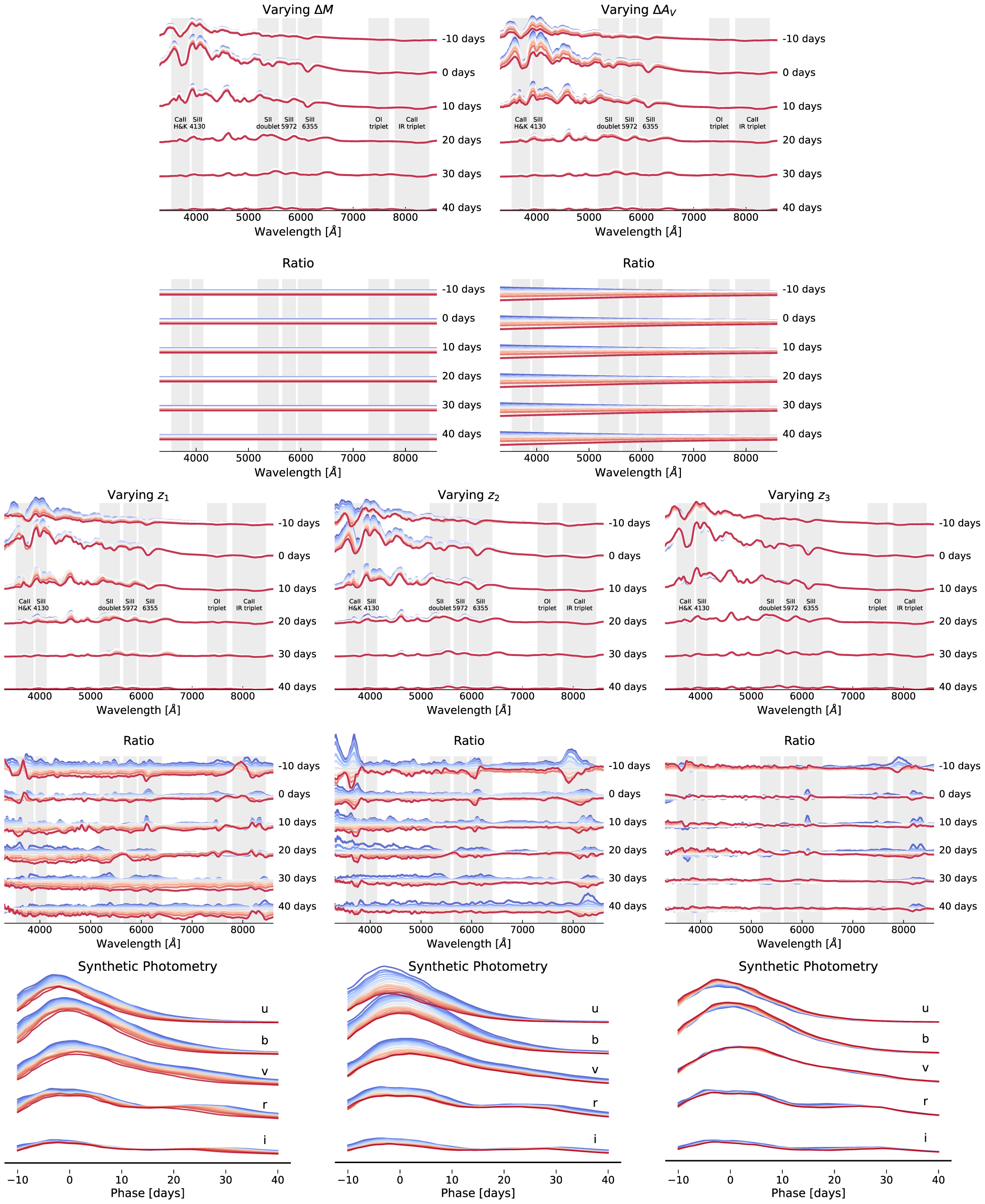
In Figure 2 we demonstrate how separately varying each latent parameter from their mean values in a three nonlinear latent dimensional model affects the reconstructed spectra. We find that the latent parameters have each encoded unique spectral information. The first and second dimensions by design were restricted to learning physical components of the model, where the former dimension encodes the extrinsic amplitude ΔM, and the latter is the time-independent color law relative extinction coefficient ΔAV . The remaining dimensions are free to learn any spectral variations that exist in the SN Ia population used for training. For the specific model shown here, we find that the z1 dimension seemingly resembles a combination of an amplitude multiplication correlated with certain absorption/emission features and a brighter-slower effect. The z2 and z3 intrinsic latent dimensions focus more on details of the absorption/emission features and spectral tilt. We note that unlike a PCA decomposition where components are ranked by the variance they explain, our autoencoder has no such constraint, and the intrinsic latent parameters are free to learn any modes of spectral diversity. The fact that the first intrinsic latent parameter happened to result in the most apparent modifications to the reconstructed spectra is a coincidence.

Figure 2. Generative sampling of SN Ia spectra as a function of phase, individually varying each latent dimension of a PAE model with two extrinsic (ΔM, ΔAV ) and three intrinsic nonlinear (z1, z2, z3) parameters, while keeping the other latent variables fixed at their mean values. The top panels of each set show the spectra with a constant offset in luminosity, while the bottom shows the ratio from the mean. For the nonlinear parameters, we also display the resulting synthetic photometry. Blue lines are values lower than the mean, transitioning through red for values higher than the mean.
Download figure:
Standard image High-resolution imageThe key difference between our nonlinear PAE model and a linear PCA analysis is that the latent dimensions of the PAE are both non-independent and nonsymmetric around the mean. We can see clearly from Figure 2 that the effects of a latent value smaller than the mean (blue) are not simply the inverse of a latent value larger than the mean (red) but describes independent information. This allows for more information to be encoded within a single dimension in comparison to PCA, where each dimension is simply a multiplier in front of a tempo-spectral component (i.e., x1 M1(t, λ) in the SALT2 model). Additionally, as the latent parameters are passed through a number of nonlinear layers of the decoder, their effects on the reconstructed spectra are not limited to the spectral variations of the independent z1 and z2 dimensions but can interact in highly nonlinear ways to produce more complex spectral features than those shown here. We show a model with three nonlinear parameters for visualization purposes, but the method can be increased to any dimensionality.
5.2. Accuracy of PAE Data Reconstructions
While we demonstrated that varying latent parameters of the PAE captures a number of complex spectral and temporal features, the key to using the model is its accuracy in modeling the SN Ia observations in the training and test sets. In Figure 3 we compare the SALT2 and PAE reconstructions of the data for two SNe from the test set. We chose to display an SN with many observed spectra and a low level of observational noise (left) and an SN with only a few observations, with none before peak brightness, and an increased observational noise level (right). These two examples demonstrate the diversity of objects in the data set and are a representative display of the performance of both the SALT2 and PAE models.

Figure 3. Top: PAE reconstruction (red) and best-fit SALT2 model (blue) of two SNe from the test set (black). For visualization purposes, the spectra in the top panels have been shifted vertically by a constant factor of the observation time. Bottom: corresponding best-fit PAE model parameters and their errors determined from HMC.
Download figure:
Standard image High-resolution imageWe find that the PAE reconstructions are highly accurate over the entire observation range from −10 to +40 days, even for samples that have highly nonuniform time sampling. In comparison to the SALT2 best-fit spectra, we see a better fit overall, both on the amplitude offset and on the matching of absorption and emission features on the spectra, particularly the Ca ii H&K, Si ii, and OI features at ∼3950 Å, ∼6150 Å, and ∼7800 Å, respectively. For SNe Ia with abnormally large luminosity at early times (e.g., Nordin et al. 2018), we find that the PAE reconstruction still matches the observations to high accuracy, while the SALT2 model fails to capture the spectral diversity of these types.
The accuracy of the reconstructions of the PAE model depends on the number of latent dimensions used. Too few dimensions do not allow for the full spectral variability of the SNe time series to be expressed, while too many dimensions can allow the model to improve the fit on the training data, with no improvement of the test data. By training multiple autoencoders, each with a different number of intrinsic nonlinear latent parameters, we studied the optimal latent dimensionality for reconstruction quality. Using the same AE architecture and multistage training procedure described in Section 4 we varied the dimensionality of the latent space from two to eight. When referring to the dimensionality of the latent space, we count only the model parameters that capture intrinsic and extrinsic effects and do not include the time shift relative to the SALT2 fits, Δp.
To quantify the quality of the model reconstructions, we report the level of unmodeled dispersion—the additional dispersion beyond the observational uncertainty required to explain the variance of the reconstructions and the data. This is determined by modeling the observed flux fobs as

and fitting for the maximum likelihood of the unmodeled dispersion σi . We report this value in magnitudes for each wavelength, binned in 5 day intervals, and show the results as a function of dimensionality in Figure 4.

Figure 4. Unmodeled dispersion—the additional dispersion beyond the observational uncertainty required to explain the variance of the reconstructions and the data (Equation (12))—of SALT2 and our PAE model with increasing dimensionality. The dispersion is measured in five-day intervals for the training data (top) and on the unseen test data (bottom). Beyond three nonlinear dimensions (z1, z2, z3), plus extinction (ΔAV ) and a free amplitude scaling parameter (ΔM), we found no improvement in the test sample and thus do not display the additional panels here.
Download figure:
Standard image High-resolution imageWe find that our PAE outperforms the standard SALT2 model at all wavelengths and observation times and that increasing the latent dimensionality continues to decrease the unmodeled dispersion across the time and wavelength range up until three nonlinear latent parameters (z1, z2, z3), after which it flattens to show no additional improvement in the test set. The dispersion near the Ca ii H&K and Si ii lines (∼3950 Å, ∼6150 Å) and near the Ca NIR triplet at ∼8100 Å shows the most significant improvement when increasing the nonlinear latent dimensionality. This clearly demonstrates that additional components describing the intrinsic variations of the SN Ia population can learn increasingly complex spectral and temporal features. The dispersion between ∼6500 and ∼7750 Å remains at ∼0.05 mag, as this region has little to no spectral features that vary between SNe. We find that the unmodeled magnitude dispersion near peak brightness is on average the lowest and increases at later times. Between 30 and 40 days after peak brightness we find that the dispersion is larger than that near the peak. The dispersion is higher even in spectral regions not associated with strong spectral features, suggesting that the uncertainty is somewhat underestimated for these very faint spectra. Integrating the test set over a B-band bandpass, we find that the SALT unmodeled dispersion near peak brightness is 0.128 mag, compared to a PAE value of 0.056 mag—a factor of 2.28 larger.
We select the three nonlinear latent dimension model as optimal for modeling the data, and as we will show below, it also returns the lowest magnitude residuals. We examine the best-fit model parameters in Figure 5. We note that the parameter values shown are those found by finding the minimum of the log posterior through HMC and not simply the encoded values of each SN. This ensures that the full parameter space has been explored and thus the variations of any parameter are not artificially small due to any limitations of the encoder. From visual inspection, we find that the magnitude residual contains no noticeable correlations with the other model parameters, confirming that our multistage training setup and correlation penalty have ensured that the intrinsic model parameters have learned clear correlations between the intrinsic luminosity and spectral and/or temporal features of SNe Ia. Given that the dimensionality of the non-ΔM parameters is large, it is possible that small correlations between these parameters and the magnitude residual remain. If so, these correlations could be uncovered with an additional nonlinear model, which could then be used to explain and reduce the extrinsic magnitude such as in the SALT2 or the Twins Embedding analysis. Initial investigations with a fully connected neural network trained on the latent parameters of the training set did not reduce the extrinsic magnitude dispersion when applied to the test set. We also find that the average time shift relative to the SALT2 fit, Δp, is within approximately half a day and is consistent with the uncertainty of the SALT2 fits and that the standard deviation of ΔAv is 0.132. A small number of SNe have time shifts of a few days relative to the SALT2 best fits. These are mostly SNe with no observations near or before peak brightness.

Figure 5. Best-fit PAE parameters for all SNe with a redshift greater than 0.02. The Pearson correlation coefficient r is shown in the top right of each panel.
Download figure:
Standard image High-resolution imageFigure 6 compares the best-fit PAE parameters to the SALT2 and the Twins Embedding models described in Section 2. As expected, we find a high degree of correlation between the magnitude residuals (ΔMSALT2, ΔMTwins, ΔMPAE) and the color ( ) between the three models, although there is a nonzero scatter. We find that the magnitude residuals cover a similar range of values, while the relative extinction inferred by the Twins Embedding covers a larger range of values than that of our PAE. This larger range is likely due to the multiple steps required to perform the Twins Embedding. Rather than train all parameters simultaneously as for the PAE, the Twins Embedding magnitude and extinction are fit first in the two-parameter RBTL step, and thus,
  is forced to simultaneously explain both the extinction and any intrinsic color-like effects. Alternatively, the PAE simultaneously learns all intrinsic and extrinsic parameters, and the intrinsic latent parameters (z1, z2, z3) can learn any color-like features that happen to be correlated with spectral or temporal features. If we instead allow the PAE to learn only a magnitude and extinction, we find that the best-fit extinction values are nearly equivalent to those reported by the Twins Embedding.

Figure 6. PAE parameters compared to SALT2 and the Twins Embedding/RBTL for overlapping SNe with a redshift greater than 0.02. The Pearson correlation coefficient r is shown in the top right of each panel.
Download figure:
Standard image High-resolution imageWe find a clear correlation between our z1 parameter and the x1 parameter of SALT2 and various correlations between our latent space and the latent Twins Embedding parameters (z1 → ξ2, z2 → ξ1, z3 → ξ3).
5.3. Simulating New SNe Ia
The generation of new SN samples consistent with the data is straightforward with a probabilistic autoencoder. We simply sample a random latent vector u from a unit Gaussian, pass this through the normalizing flow to get the sample in autoencoder latent space z , append the desired observation times and magnitude offset ΔM, and pass this through the decoder to yield a new spectral time series. By the probabilistic nature of the normalizing flow Gaussian latent space u , the distribution of generated samples corresponds to the density of similar samples in the training data set—significant outliers will be rare, while "average" spectra will have a higher probability of being generated.
5.4. Detecting Outlying SNe
The PAE framework allows for an effortless determination of data density in both z and u space, which are simply related through the Jacobian determinant of the normalizing flow. Samples residing in low-density regions of the latent space are less similar to other SNe, while those in high-density regions are more similar to others. Therefore, by selecting SNe by the density of their latent representations, p( z ), we can pull out outliers or common samples for further inspection. Low density does not mean that these SNe are more poorly fit by the PAE—we do not find that either the reconstruction error or magnitude residual depends on density—only that the latent parameters and hence corresponding spectral characteristics are more unique.
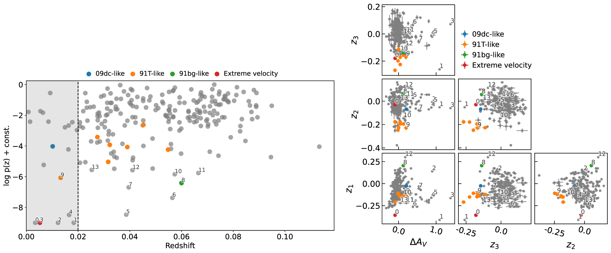
Figure 7 shows the density as a function of redshift for all SNe (left), calculated from their best-fit latent parameters. We find no distributional shifts between SNe in the training and test sets, so we include all 228 SNe here. It is clear that there are a few SNe residing in low-density regions of the latent space—i.e., with the smallest values of log p( z ). ΔAV is included, and because strongly reddened SNe Ia can easily become isolated in that dimension, low values for log p( z ) can result. This explains all the cases with log p( z ) < 10−8. A number of these are at low redshifts, but as we have excluded the amplitude parameter ΔM from the density calculation as described in Section 3.2, the density estimation should be immune to the effects of peculiar velocities on amplitudes.

Figure 7. Best-fit PAE latent parameters with peculiar SNe Ia displayed as colored markers. The left panel shows the density of each SN as a function of the redshift, while the right panel displays where the SN resides in each latent dimension. We annotate the 14 lowest-density examples in order to enable comparisons between the left and right panels.
Download figure:
Standard image High-resolution imageFor a small number of SNe in our data set, we have external labels specifying peculiar subtypes, including 91T-like, 91bg-like, and 09dc-like, which we highlight with different colored markers. We find that the best-fit PAE model parameters for these SNe are in regions of lower than average density, which is expected given that they belong to rare subpopulations. As the number of SNe of a certain subtype grows, their region of the latent space becomes well populated, and thus a low likelihood is more effective at finding individual rare SNe, such as the 91bg-like example, rather than whole subpopulations such as the 91T-like. For subpopulations, it is better to examine clusters in various regions of the latent space.
A closer inspection of individual dimensions of the latent space (right panel) shows that low-density SNe are not necessarily peculiar among all dimensions; rather, their peculiar features are often isolated in a specific dimension, such as large values of ΔAV , as noted above, or low values of z2 or z3. We annotate the 14 lowest-density examples in order to enable comparisons between the left and right panels. We find that five of the six lowest-density examples are SNe with high extinction and are mostly at low redshifts. The large extinction results in a relatively small transmitted flux, so perhaps similar SNe Ia at high redshift are simply below the flux detection threshold. We also find a clear cluster of 91T-like SNe with low values of both z2 and z3, demonstrating that the PAE is a valuable tool for population studies of SNe. Beyond the five low-redshift SNe with high extinction, we find no clear population shifts as a function of redshift.
5.5. Cosmological Distance Measurements
The application with perhaps the most scientific utility is the determination of the magnitude residual for each SN, which is the key factor for determining the distance accuracy. As explained in Section 4 the three-stage training and correlation penalty term encouraged our PAE model to separate the extrinsic magnitude component, which is uncorrelated with features of the spectral time series, from any amplitude-like modification that is correlated with intrinsic spectral features or temporal evolution. Thus, the extrinsic magnitude residual ΔM is directly fit for during the posterior analysis phase of our analysis, and we do not require any additional steps to uncover correlations between model parameters and magnitude residuals in order to perform magnitude standardization. This differs from the methodology employed in the SALT2 and Twins Embedding models that we compare to, which employ an additional linear (SALT2) or nonlinear (Twins) model to predict the magnitude given the model parameters, and remove this predicted value to obtain a final magnitude residual. Although the PAE model parameters may end up having some small remaining correlations with ΔM that can be exploited to explain the magnitude residuals, we do not perform any magnitude standardization for the results shown here. Whether magnitude standardization benefits from learning correlations during model training, rather than determining them after model training is completed, is not obvious a priori but is nevertheless an interesting topic for future investigation.
As outlined in Section 3.2 we marginalize over (ΔM, u , Δp) for each SN Ia to obtain the final best-fit model parameters and their uncertainty through HMC starting from the best-fit MAP parameter, using the mean and percentiles of the posterior samples as the mean and error on the best-fit parameters. To enhance the predictive performance and error estimation on the physical SN parameters inferred by a single PAE model, we use the weighted mean and variance calculated from the results of 10 separate models. Each model is trained in an identical fashion on the training set with the procedure described above but using a different random seed to initialize network weights. On the ΔM parameter for all models, we include a peculiar velocity error component, assuming a velocity of vpec = 300 km s−1. 23
We first studied the magnitude residuals as a function of the latent dimensionality of the model, finding a clear decrease in the magnitude residual for both the training and test sets as we increase the latent dimensionality from zero to three nonlinear intrinsic parameters. Similar to the intrinsic dispersion results of Figure 4, we find no statistically significant improvement when increasing beyond a model with three nonlinear parameters (i.e., (z1, z2, z3) plus extinction and an amplitude scaling). This is in agreement with Boone et al. (2021a, 2021b), who find quickly diminishing returns when expanding beyond three nonlinear intrinsic model parameters. From this investigation, we determined that this model is optimal for explaining the diversity of SNe Ia given our data set and again restrict to this model for the following results.
In Figure 8 we compare the PAE magnitude residuals to those derived by SALT2 and Twins Embedding analyses for SNe Ia in common—137 SNe in the training set and 44 in the test set. Of this overlapping fraction, 96 of the training and 32 of the test were part of the final Twins cosmological distance analysis. We display both the (unweighted) rms (denoted σ) and the normalized median absolute deviation (NMAD) of the magnitude residuals. While both statistics are similar, the NMAD is less susceptible to large outliers. We show the rms and NMAD for SALT2, Twins, and PAE over the subset of SNe that overlap with the ones used in the final Twins Embedding cosmological distance analysis.

Figure 8. Magnitude residuals of SNe from the training (top) and test (bottom) sets, including the component from peculiar velocities. Both the SALT2 and Twins Embedding results are obtained from a linear (SALT2) or nonlinear (Twins) magnitude standardization procedure, while our probabilistic autoencoder has been trained to explicitly separate the extrinsic magnitude from the intrinsic SNe luminosity and thus requires no standardization. Solid data points are those used in the final Twins Embedding cosmological distance analysis, while data points with some transparency are the remaining overlap between our data and the full Twins Embedding data set.
Download figure:
Standard image High-resolution image
It is important to note that each analysis had somewhat different subsets of SNe Ia available for development and training, especially given the small number of data samples available, which theoretically could cause a small number of outlying SNe that exist in one data set but not another to considerably alter model training. Thus although this analysis facilitates a comparison of the magnitude standardization capabilities of the three models, the magnitude residuals we report inevitably reflect a combination of the strength of the method at explaining the diversity of SNe Ia coupled with signatures of the specific data used for model training—it is impossible to disentangle model implementations from subtle effects introduced by the different training data. However, by focusing only on the SNe that do overlap between the different analyses, we attempt to mitigate any such differences.
For individual SNe Ia, we see consistent results across all models, specifically the low-redshift objects with large magnitude residuals resulting from significant peculiar velocities, which helps to validate the fitting procedure employed in our analysis. Our model was trained using a minimum redshift cut of 0.02 and thus was not trained using any objects with significant redshift contribution due to peculiar velocity, but by excluding the ΔM parameter from the normalizing flow we have included no prior on the extrinsic amplitude and it is allowed to freely vary to any value that best fits the data.
We find that our PAE obtains significantly smaller magnitude residuals than the SALT2 model and shows a magnitude residual similar to that of the Twins Embedding analysis. None of the SNe in our data set were used for training the SALT2 model, such that the test set illustrates an unseen sample and thus a true test sample performance for both SALT2 and our PAE. The samples we display for Twins will include both samples used for training and those used for testing. For the PAE we find a smaller magnitude residual for the training set in comparison to the test set, which is commonly found in the generalization of deep neural networks to unseen samples, but the difference is not statistically significant. This does not equate to model overfitting, in which continuing to improve the fit on the training data comes at a cost of decreasing performance on unseen test data. As discussed in Section 4.3 we find no evidence for this, and the test error continues to decrease until flattening. Had we had a larger training sample, we would have separated out a validation set and stopped training when the error on this set stopped decreasing, but we did not want to further reduce the number of available training samples by separating out a validation set in addition to the test set. This choice of not performing early stopping during training was made to ensure that the model remained blind to the test set.
We tabulate the final magnitude residuals for all methods in Table 1. While we do not have the same SNe in our data set that were used in Boone et al. (2021b), we find that the statistics we report for their results are similar to those quoted in their paper of NMAD = 0.83 ± 0.010 and σ = 0.101 ±0.070 over the full sample of 134 SNe that passed their data cuts. To approximate removing the component of the magnitude residual stemming from peculiar velocities, we assume a 300 km s−1 velocity for each SN, which contributes an added dispersion of 0.053 mag. We subtract this from the rms in quadrature. The uncertainty reported on the rms and NMAD is determined by bootstrap resampling (Efron 1979) of the magnitude residuals.
Table 1. Standardization Performance for Methods Presented in This Work, Showing the NMAD, rms, and an Estimate of the rms with the Peculiar Velocity Removed (see Text for Details)
| Data Sample | Statistic | SALT2 | Twins Embedding | PAE |
|---|---|---|---|---|
| NMAD | 0.099 ± 0.013 | 0.083 ± 0.014 | 0.060 ± 0.010 | |
| Train | rms | 0.126 ± 0.012 | 0.101 ± 0.009 | 0.074 ± 0.010 |
| rms w peculiar velocity removed | 0.115 ± 0.012 | 0.087 ± 0.009 | 0.052 ± 0.010 | |
| NMAD | 0.152 ± 0.039 | 0.087 ± 0.019 | 0.084 ± 0.023 | |
| Test | rms | 0.166 ± 0.022 | 0.095 ± 0.012 | 0.091 ± 0.010 |
| Peculiar velocity removed | 0.157 ± 0.022 | 0.079 ± 0.012 | 0.074 ± 0.010 | |
Note. The significant difference between the train and test performance of the SALT2 model stems from the random assortment of SNe into each set, which combined with the small number of total samples happened to place a higher fraction of large SALT2 magnitude residual SN into the test set. This is reflected in the increase in uncertainty reported on the rms and NMAD, determined by bootstrap resampling (Efron 1979).
Download table as: ASCIITypeset image
The agreement between the Twins Embedding analysis and our PAE is interesting given that the data products used to perform the analysis are quite different. The Twins Embedding models the diversity of SNe Ia only at maximum light, interpolating a max light spectra using observations from within (−5 days, +5 days) from peak brightness. Therefore, any information from observations outside of this window is not included in the Twins Embedding analysis, while the PAE is allowed to learn the full temporal evolution in addition to the diversity at maximum light. Nevertheless, the magnitude residuals between the two methods are similar, seemingly pointing toward observations near peak brightness being the most important for standardization, similar to that noted by Fakhouri et al. (2015) and Léget et al. (2020). To investigate the PAEs reliance on observations near peak, we perform an equivalent posterior analysis while masking any spectra within a (−5 day, +5 day) range from maximum brightness. We find that when only using spectra outside of this range the NMAD and rms increase to 0.080 ± 0.014 and 0.112 ± 0.011 on the training set, and 0.092 ± 0.032 and 0.135 ± 0.017 on the test set. This magnitude residual when only using observations away from peak brightness, while still an increase over using the full time series, demonstrates that the PAE does not require any observations near peak brightness to still obtain relatively small magnitude residuals and implies that the intrinsic brightness of the SNe can be determined from spectra at any date from −10 to +40 days relative to peak brightness.
6. Discussion and Conclusions
The goal of this paper is to develop a single framework for SN Ia data analysis, developing a data-driven model that can be used for all of the downstream tasks, including posterior analysis of all of its parameters including the distance modulus, anomaly detection, and realistic SN Ia spectro-temporal simulations. Our approach is a physically parameterized probabilistic autoencoder (PAE) to model Type Ia SN spectral evolution. We showed that the model, trained directly on the data without any data cuts, separately learns both intrinsic variation and extrinsic variation (dust and distance modulus) of SN variability and can model the data to very high accuracy. We introduced a multistage training procedure, which, with the addition of a correlation penalty term between the model parameters, disentangles extrinsic magnitude changes due to peculiar velocities from the portion of the intrinsic luminosity of the SNe that correlated with optical spectral and/or temporal features.
The disentanglement of intrinsic and extrinsic effects during training is novel to this work. Usually, the discovery of correlations between model parameters and magnitude dispersion composes an additional "magnitude standardization" step after the model is trained, which requires another linear or nonlinear model and thus introduces another set of errors that need to be propagated through to the final constraints. In contrast, in our approach, all of the training is done once. We demonstrate that the intrinsic scatter, even when inflated by the peculiar velocity dispersion, can be as low as 0.1 mag, which bodes well for peculiar velocity measurements with local SNe.
Both our analysis and that of Boone et al. (2021b) show that SNe Ia inhabit a three-dimensional parameter space (see Rubin 2020 for a more complete discussion of this concept). Physical modeling of SN Ia explosions involves many more parameters (Hillebrandt & Niemeyer 2000), e.g., so our results imply the presence of strong correlations among these parameters. The z1,2,3 space presented here offers an efficient means of comparing SN Ia model results with real SNe Ia. Significant challenges remain in producing high-fidelity spectral models of SN Ia explosions (see Röpke et al. 2012), as even small changes in the modeling of radiative transfer produce strong effects on model spectra. More mature physical models can eventually be efficiently compared in our z1,2,3 space.
We release all codes, and the trained models, at https://github.com/georgestein/suPAErnova.
M.R. has received funding from the European Research Council (ERC) under the European Union's Horizon 2020 research and innovation program (grant agreement No. 759194—USNAC) This work was supported in part by the Director, Office of Science, Office of High Energy Physics of the US Department of Energy under contract No. DE-AC02-05CH11231. Support in France was provided by CNRS/IN2P3, CNRS/INSU, and PNC and French state funds managed by the National Research Agency within the Investissements d'Avenir program under grant reference numbers ANR-10-LABX-0066, ANR-11-IDEX-0004-02 and ANR-11-IDEX-0007. Additional support comes from the European Research Council (ERC) under the European Union's Horizon 2020 research and innovation program (grant agreement No. 759194–USNAC). Support in Germany was provided by DFG through TRR33 "The Dark Universe" and by DLR through grants FKZ 50OR1503 and FKZ 50OR1602. In China support was provided by Tsinghua University 985 grant and NSFC grant No. 11173017. Some results were obtained using resources and support from the National Energy Research Scientific Computing Center, supported by the Director, Office of Science, Office of Advanced Scientific Computing Research of the US Department of Energy under contract No. DE-AC02-05CH11231. We also thank the Gordon & Betty Moore Foundation for their support.
Footnotes
- 23
This is the prediction from linear perturbation theory (see, e.g., Hui & Greene 2006).