CERN Accelerating science

 
On the left is a sketch (not to scale) illustrating the basic operating principle of the PLT: a track originating from the CMS interaction point passing through a single PLT telescope will produce a triple coincidence. The center of the first plane is 4.45\cm from the beam axis, with the other two planes slightly farther away in the radial direction to match the slope of tracks coming from the IP. This produces a pointing angle of 1.15$^{\circ}$ between the beam axis and the line connecting the centers of each plane. On the right is a sketch illustrating two possible sources of accidentals in the PLT: the solid green lines show a combinatorial background, where hits from two tracks that do not individually pass through all three planes produce a triple coincidence together, while the dashed red line shows a track from a noncollision source, in this case beam-induced background, passing through all three planes of a PLT telescope.
Schematic of the arrangement of the PLT telescopes, numbered by position, for the $-z$ side (left) and the $+z$ side (right), viewed looking towards the IP. The ``near'' side is the side closer to the center of the LHC ring.
A schematic of the readout scheme for a single PLT quadrant, showing the data flow from the individual ROCs through the port card and OMB to the FEDs and FEC on the back end. The FEC and pixel FED are shared among all four quadrants, while one fast-or FED serves two quadrants.
Closeup of an assembled cassette, with the gray cooling tubes visible in the foreground, the hybrid boards behind (one is visible at the center of the picture, carrying the silicon sensor visible as the silver rectangle), and the HDIs running horizontally in the background. The port card is just visible to the left of the ribbon in the foreground.
A demonstration of the active area alignment procedure in 2016, using data from LHC fill 4892. The color scale indicates the occupancy (number of hits) in each pixel. The center plane (center) uses the normal active area, while the outer planes (left and right) use a larger active area, allowing the image of the center plane to be clearly visible.
The XdY plots for the second plane (ROC 1) in telescope 7 for fill 4444 in 2015, showing the profiled distribution of the $y$ residual distance between the hit position and the fitted track as a function of the $x$ coordinate of the track at the plane. The three plots show the three stages of the alignment: (left) before alignment, assuming that the second and third planes are in exactly the design position relative to the first plane; (center) after the rotational correction, where the position of the plane has been rotated using the slope of the fitted line in the first plot (and similarly for the third plane); (right) after the translational correction, when the alignment procedure is complete. The blue line shows the fit used to determine the slope in the first plot, and the offset in the second plot.
Alignment vs. time for a single PLT telescope (channel 10) for nine different fills in 2015, where brackets denote fills in which the CMS magnet was off. The alignment is described by six parameters: rotation ($\Delta\theta$), translation in $x$ ($\Delta x$), and translation in $y$ ($\Delta y$) of ROC 1 relative to ROC 0, and the same three quantities for ROC 2 relative to ROC 0. The nominal value for each of these is zero, except for $\Delta y$, which has a physical nonzero value, because of the 1.15$^\circ$ angle between the beam axis and the center line of a telescope. The left plot shows the absolute alignment values, and the right shows the difference of these values (designated by $\delta$) compared to their average.
Measured PLT accidental rate, as a function of SBIL, for selected fills in 2015 (\cmsUL) and 2016 (\cmsUR). For 2015, a linear fit for each fill is shown; in 2016, for clarity, only the linear fit for fill 5151 is shown. The apparent increase in the accidental rate at very low luminosities in 2015 is because of the larger relative contribution from beam-induced background, as discussed in the text. The bottom plot shows the evolution of the slope of the per-fill accidental rate fit over the course of 2016, where the black line shows a linear fit to the results.
Maximum likelihood fit to the slope distribution from fill 4979 in 2016 with an instantaneous luminosity of approximately 6\ten{33}\percms. The dotted green curve represents the component from the distribution at VdM luminosity, the dashed red curve represents the additional accidental contribution at higher luminosities, and the solid blue curve is their sum.
Measured PLT accidental rate for a typical LHC fill, as a function of SBIL, for different active areas. The 2015 active area was 28 columns${\times}$41 rows in the central plane and 34 columns${\times}$50 rows in the outer planes, and the selected active area for 2016 was 24 columns${\times}$36 rows in the central plane and 26 columns${\times}$38 rows in the outer planes. We observe that the size of the ``fringe'' area (the extra area in the outer planes compared to the central plane) has a substantial effect on the accidental rate.
Average sensor efficiencies for three telescopes as a function of integrated luminosity in 2015--17, for channels 8 (\cmsLeft), 10 (center), and 12 (\cmsRight). The dashed lines indicate points at which the bias voltage used for the sensors was changed. The uncertainties in the efficiency values are too small to be visible in this plot.
Pulse height distributions for fill 6035 in 2016, divided into 1-hour intervals, where each color represents a separate interval. Since each interval may not contain the same number of events, each individual histogram is normalized to a total of 1.
\cmsLeftCap: Pulse height distribution for a single ROC in a single LHC fill before (solid red line) and after (dashed blue line) the triple coincidence requirement is applied. \cmsRightCap: Pulse heights only for events in the leading bunch of a train (dashed blue line), and only for events corresponding to the first empty BX after a train (solid red line). In both plots, all histograms are normalized to unit area. These distributions are from a 2018 fill, where the hit thresholds on the ROCs were lower than in 2016 (Fig.~\ref{fig:phintervals}).
Raw (orange diamond) and normalized (blue square) rates at each HV set point for channel 10 in a 2018 scan. The vertical line indicates the calculated \Vmax. We observe some nonuniform behavior at low HV values, likely due to time walk effects.
Calculated \Vmax derived from HV scans as a function of integrated luminosity for four selected PLT channels: channel 3 (upper left), channel 10 (upper right), channel 12 (lower left), and channel 14 (lower right). The dashed vertical lines indicate changes in operating conditions, with the rightmost denoting the change in the ROC thresholds ($\Delta$threshold) and the rest denoting a change in the applied HV. In general, an upward trend is visible. The change in the ROC thresholds resulted in a smaller voltage being necessary.
The \cmsLeft two plots show an occupancy map for a single ROC during a period of good operation and the corresponding values of the 31 variables used as input to the $k$-means clustering. The \cmsRight two plots show similar plots for a period when the pixel data was not correctly decoded, resulting in line errors in the occupancy plot.
Measured PLT background rate as a function of time, using the precolliding BX method, in beams 1 (red) and 2 (purple) as compared to the BCM1F background in beams 1 (blue) and 2 (green). This study was carried out in fill 5005, a special LHC fill in which background levels were deliberately increased by injecting gas into the beam pipe. The lower panel shows the vacuum pressure, as measured by three pairs of gauges located where the gas was injected, the first pair 148\unit{m} left (L) and right (R) of the CMS interaction point, and the other two pairs 58 and 22\unit{m} on either side.
Ratios of PLT to HFOC instantaneous luminosity, as a function of SBIL, in the high-pileup fill 7358 (red line) and the reference fill 6854 (blue line), for a single PLT channel (channel 13). The left plot shows a single isolated bunch (BCID 536 in fill 7358 and BCID 823 in fill 6854), the center plot shows a leading bunch in a bunch train (BCID 750 in fill 7358 and BCID 62 in fill 6854), and the right plot shows the train bunch with the highest luminosity (BCID 1648 in fill 7358 and BCID 63 in fill 6854). The shaded bands indicate the uncertainty in the linear fit for each fill.
Measured slope of the PLT/HFOC ratio as a function of BCID for isolated bunches (the two bunches at the left in the blue background), leading bunches (the two bunches on a light red background), and train bunches (other bunches) for PLT channels 12--15 in the high-pileup fill 7358.
The position of the beamspot mean in global $x$ (\cmsLeft) and $y$ (\cmsRight) coordinates vs. fill numbers. The coordinates are estimated from the straight line fits in the $x$-$z$ and $y$-$z$ projections when extrapolated to $z=0$. The distributions of the coordinates are fit to double Gaussian functions. The dashed black line indicates the start of the heavy ion run. The different marker colors and shapes indicate groups of fills for which the beamspot position is relatively constant.
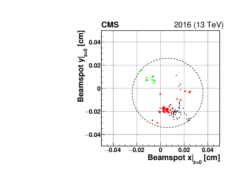
The position of the mean beamspot in global $x$ and $y$ coordinates. The red squares indicate fills from the period of stable beamspot position, shown by the red squares in Fig.~\ref{fig:BSevolution}. The green dots indicate a secondary position that is offset from the red cluster of positions by about 150\mum in $x$ and 300\mum in $y$. Theses fills occur at the beginning and end of the 2016 $\Pp\Pp$ run period. The black diamonds correspond to other fills. The dashed circle represents the overall range of beamspot position during 2016. It is centered at $x=60\mum$ and $y=-40\mum$ and has a radius of 300\mum.
Normalized PLT rates (dots) and the resulting fitted Gaussian scan curves (black curves) as a function of the beam separation ($\Delta$) for a single colliding bunch, for scans in the $x$ (left column) and $y$ (right column) direction. The top row shows results from a scan pair in the 2017 VdM program in LHC fill 6016~\cite{CMS-PAS-LUM-17-004}, using a double Gaussian fit (the two individual components are shown by the red and green curves), and the bottom row shows results using a scan pair in the 2018 VdM program in fill 6868~\cite{CMS-PAS-LUM-18-002}, using a single Gaussian fit. The background subtraction procedure described in the text has been applied to the raw data before the fit. The lower panel in each plot shows the residual difference between the fit and data, in units of the uncertainty $\sigma$. The statistical uncertainty in the $\Sigma$ values from the fit is 0.4--0.5\%.
\cmsLeftCap: Efficiency corrections determined from the 2017 emittance scan analysis as a function of the integrated luminosity over the course of the year. \cmsRightCap: Linearity measured for a single fill (fill 6325), showing the results from emittance scans at the beginning (right side) and end (left side) of the fill for leading (blue squares) and train (red circles) bunches. The fits for each type of bunch are shown by the lines, and the resulting slopes are shown in the legend.
The average sensor efficiency for channel 12 obtained with the track-hit method (dashed red line) and the per-telescope efficiency measured from the analysis of the emittance scan data (dotted blue line), with their ratio (solid black line) shown in the lower pane, as a function of time in 2017. Both efficiencies are normalized to 1 for the first fill considered. The uncertainties in the individual values are too small to be visible.
\cmsLeftCap: Efficiency of PLT relative to RAMSES over the course of 2016, where each point represents a single fill. \cmsRightCap: Linearity of PLT relative to RAMSES over the course of 2016, where each point indicates the fitted nonlinearity and its uncertainty for a single fill. The red lines show the fit functions that are used to obtain the final efficiency and linearity corrections for 2016. The uncertainties in the efficiency measurements are too small to be visible on the plot.
Top: PLT per-channel luminosity values as a function of time for fill 6860 in 2018, showing the total (\ie, over all BXs) instantaneous luminosity as measured by the PLT detector. Bottom: Per-channel luminosity values for the same fill after applying the per-channel weights described in the text to correct for differing linearity and efficiency.
Ratio histograms for different luminometer pairs during 2018. Each entry represents a period of 50 lumi sections, weighted by the luminosity in that period. Left: HFOC/PLT; middle: PCC/PLT; right: RAMSES/PLT.
Slope distribution measuring the relative nonlinearity between different luminometer pairs during 2018: (left) HFOC/PLT, (middle) PCC/PLT, (right) RAMSES/PLT.
Left: Luminosity obtained from track reconstruction (green crosses) vs. PLT fast-or luminosity (blue squares) and forward hadron calorimeter luminosity (HFOC, red circles) for fill 5109 as a function of time. The track luminosity is cross-calibrated to the HFOC luminosity at the beginning of the fill. Right: Ratios of the track luminosity to the fast-or and HFOC luminosities as a function of SBIL measured by the luminometer in the denominator of the ratio.
Scan curves using the track luminosity data during the fourth VdM scan pair in the 2017 VdM fill (fill 6016) for a single colliding bunch (BCID 1112) in the $x$ (left) and $y$ (right) directions. The extracted $\Sigma$ and its statistical uncertainty are also shown.
Top: Measured $\Sigma_x$ (blue squares) and $\Sigma_y$ (red circles) values as a function of BCID for the track luminosity measurement. Bottom: Measured \sigmavis value as a function of BCID. The red line indicates the fitted average over all bunches.