CERN Accelerating science

Sketch of a \DzKK to \DzRS matching.

Matched versus original transverse momenta for the matching of a $K^-$ to a $\pi^-$ particle, related to the $\ycp^{CC}$ measurement. The red line represents the requirement applied to the data sample, where candidates below the line are rejected. The plot is obtained with the 2017 \textit{MagUp} sample.

Distributions of $\Delta m$ for the (top) \DzRS, (centre) \DzKK, and (bottom) \DzPP decay channels for the combined data sample. The signal and sideband regions employed to subtract the combinatorial background are delimited by the dashed vertical lines. The sum of the fit projections are overlaid.

Distributions of $\Delta m$ for the (top) \DzRS, (centre) \DzKK, and (bottom) \DzPP decay channels for the combined data sample. The signal and sideband regions employed to subtract the combinatorial background are delimited by the dashed vertical lines. The sum of the fit projections are overlaid.

Distributions of $\Delta m$ for the (top) \DzRS, (centre) \DzKK, and (bottom) \DzPP decay channels for the combined data sample. The signal and sideband regions employed to subtract the combinatorial background are delimited by the dashed vertical lines. The sum of the fit projections are overlaid.

(Left) fraction and (right) average true $\Dz$ decay time of secondary decays as a function of the reconstructed $\Dz$ decay time, in units of the average $\Dz$ lifetime.

(Left) fraction and (right) average true $\Dz$ decay time of secondary decays as a function of the reconstructed $\Dz$ decay time, in units of the average $\Dz$ lifetime.

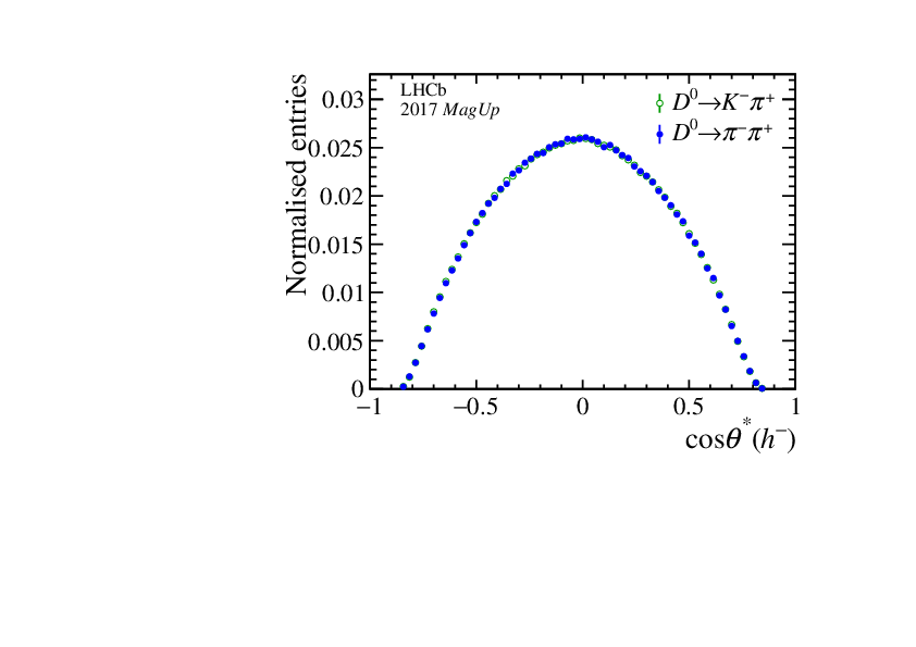
(Left) normalised distributions of the $D^0$ decay angle $\cos \theta^{\ast}(h^-)$ in the raw condition, and (right) following both kinematic matching and reweighting procedures. The distributions are shown for the (top) $\ycp^{CC}$, (middle) $\ycp^{\pi\pi} - \ycp^{K\pi}$ and (bottom) $\ycp^{KK} - \ycp^{K\pi}$ measurements. The plots are obtained with the 2017 \textit{MagUp} sample.

(Left) normalised distributions of the $D^0$ decay angle $\cos \theta^{\ast}(h^-)$ in the raw condition, and (right) following both kinematic matching and reweighting procedures. The distributions are shown for the (top) $\ycp^{CC}$, (middle) $\ycp^{\pi\pi} - \ycp^{K\pi}$ and (bottom) $\ycp^{KK} - \ycp^{K\pi}$ measurements. The plots are obtained with the 2017 \textit{MagUp} sample.

(Left) normalised distributions of the $D^0$ decay angle $\cos \theta^{\ast}(h^-)$ in the raw condition, and (right) following both kinematic matching and reweighting procedures. The distributions are shown for the (top) $\ycp^{CC}$, (middle) $\ycp^{\pi\pi} - \ycp^{K\pi}$ and (bottom) $\ycp^{KK} - \ycp^{K\pi}$ measurements. The plots are obtained with the 2017 \textit{MagUp} sample.

(Left) normalised distributions of the $D^0$ decay angle $\cos \theta^{\ast}(h^-)$ in the raw condition, and (right) following both kinematic matching and reweighting procedures. The distributions are shown for the (top) $\ycp^{CC}$, (middle) $\ycp^{\pi\pi} - \ycp^{K\pi}$ and (bottom) $\ycp^{KK} - \ycp^{K\pi}$ measurements. The plots are obtained with the 2017 \textit{MagUp} sample.

(Left) normalised distributions of the $D^0$ decay angle $\cos \theta^{\ast}(h^-)$ in the raw condition, and (right) following both kinematic matching and reweighting procedures. The distributions are shown for the (top) $\ycp^{CC}$, (middle) $\ycp^{\pi\pi} - \ycp^{K\pi}$ and (bottom) $\ycp^{KK} - \ycp^{K\pi}$ measurements. The plots are obtained with the 2017 \textit{MagUp} sample.

(Left) normalised distributions of the $D^0$ decay angle $\cos \theta^{\ast}(h^-)$ in the raw condition, and (right) following both kinematic matching and reweighting procedures. The distributions are shown for the (top) $\ycp^{CC}$, (middle) $\ycp^{\pi\pi} - \ycp^{K\pi}$ and (bottom) $\ycp^{KK} - \ycp^{K\pi}$ measurements. The plots are obtained with the 2017 \textit{MagUp} sample.

Results for (top) $\ycp^{CC}$, (centre) $\ycp^{\pi\pi} - \ycp^{K\pi}$ and (bottom) $\ycp^{KK} - \ycp^{K\pi}$. The measurements employing raw data, and following both matching and weighting conditions are shown in green, blue and red, respectively. The measurements in purple employ the fit model where the presence of secondary decays is considered. The dashed vertical lines correspond to $\chi^2$ fits, used to determine the average values other all subsamples. In the y-axis labels, the data-taking year is abbreviated with the last two digits only and the magnet polarity \MagUp (\MagDown) is abbreviated as ``Up'' (``Dw'').

Results for (top) $\ycp^{CC}$, (centre) $\ycp^{\pi\pi} - \ycp^{K\pi}$ and (bottom) $\ycp^{KK} - \ycp^{K\pi}$. The measurements employing raw data, and following both matching and weighting conditions are shown in green, blue and red, respectively. The measurements in purple employ the fit model where the presence of secondary decays is considered. The dashed vertical lines correspond to $\chi^2$ fits, used to determine the average values other all subsamples. In the y-axis labels, the data-taking year is abbreviated with the last two digits only and the magnet polarity \MagUp (\MagDown) is abbreviated as ``Up'' (``Dw'').

Results for (top) $\ycp^{CC}$, (centre) $\ycp^{\pi\pi} - \ycp^{K\pi}$ and (bottom) $\ycp^{KK} - \ycp^{K\pi}$. The measurements employing raw data, and following both matching and weighting conditions are shown in green, blue and red, respectively. The measurements in purple employ the fit model where the presence of secondary decays is considered. The dashed vertical lines correspond to $\chi^2$ fits, used to determine the average values other all subsamples. In the y-axis labels, the data-taking year is abbreviated with the last two digits only and the magnet polarity \MagUp (\MagDown) is abbreviated as ``Up'' (``Dw'').

Distributions of (left) $R^{\pi\pi}(t)$ and (right) $R^{KK}(t)$ using the full \lhcb Run~2 data set, with the results of $\ycp^{\pi\pi} - \ycp^{K\pi}$ and $\ycp^{KK} - \ycp^{K\pi}$ overlaid as the blue slopes.

Distributions of (left) $R^{\pi\pi}(t)$ and (right) $R^{KK}(t)$ using the full \lhcb Run~2 data set, with the results of $\ycp^{\pi\pi} - \ycp^{K\pi}$ and $\ycp^{KK} - \ycp^{K\pi}$ overlaid as the blue slopes.