CERN Accelerating science

The distributions of the multijet BNN discriminant used for the QCD multijet background rejection (left) and the reconstructed transverse W boson mass (right) from data (points) and the predicted backgrounds from simulation (filled histograms) for $\sqrt{s}=8\TeV$. The lower part of each plot shows the relative difference between the data and the total predicted background. The vertical bars represent the statistical uncertainties.

The distributions of the multijet BNN discriminant used for the QCD multijet background rejection (left) and the reconstructed transverse W boson mass (right) from data (points) and the predicted backgrounds from simulation (filled histograms) for $\sqrt{s}=8\TeV$. The lower part of each plot shows the relative difference between the data and the total predicted background. The vertical bars represent the statistical uncertainties.

Comparison of experimental with simulated data of the BNNs input variables $\cos(\theta_{\mu,\rm {\rm j_L}})|_\text{top}$, $\eta(\rm j_L)$, $H_{\rm T}(\rm j_1, j_2)$, and $M(\rm W,\rm {b_1})$. The variables are described in Table~\ref{tab:BNN input vars}. The lower part of each plot shows the relative difference between the data and the total predicted background. The hatched band corresponds to the total simulation uncertainty. The vertical bars represent the statistical uncertainties. Plots are for the $\sqrt{s}=$ 8\TeV data set.

Comparison of experimental with simulated data of the BNNs input variables $\cos(\theta_{\mu,\rm {\rm j_L}})|_\text{top}$, $\eta(\rm j_L)$, $H_{\rm T}(\rm j_1, j_2)$, and $M(\rm W,\rm {b_1})$. The variables are described in Table~\ref{tab:BNN input vars}. The lower part of each plot shows the relative difference between the data and the total predicted background. The hatched band corresponds to the total simulation uncertainty. The vertical bars represent the statistical uncertainties. Plots are for the $\sqrt{s}=$ 8\TeV data set.

Comparison of experimental with simulated data of the BNNs input variables $\cos(\theta_{\mu,\rm {\rm j_L}})|_\text{top}$, $\eta(\rm j_L)$, $H_{\rm T}(\rm j_1, j_2)$, and $M(\rm W,\rm {b_1})$. The variables are described in Table~\ref{tab:BNN input vars}. The lower part of each plot shows the relative difference between the data and the total predicted background. The hatched band corresponds to the total simulation uncertainty. The vertical bars represent the statistical uncertainties. Plots are for the $\sqrt{s}=$ 8\TeV data set.

Comparison of experimental with simulated data of the BNNs input variables $\cos(\theta_{\mu,\rm {\rm j_L}})|_\text{top}$, $\eta(\rm j_L)$, $H_{\rm T}(\rm j_1, j_2)$, and $M(\rm W,\rm {b_1})$. The variables are described in Table~\ref{tab:BNN input vars}. The lower part of each plot shows the relative difference between the data and the total predicted background. The hatched band corresponds to the total simulation uncertainty. The vertical bars represent the statistical uncertainties. Plots are for the $\sqrt{s}=$ 8\TeV data set.

Comparison of $\sqrt{s} = 8\TeV$ data and simulation using the SM BNN discriminant in three separate signal regions of two jets with one b-tagged (2 jets, 1 tag) (upper), three jets with one of them b-tagged (3 jets, 1 tag) (middle left), and three jets with two of them b-tagged (3 jets, 2 tags) (middle right), and in \ttbar (4 jets, 2 tags) (lower left) and \wjets (no b-tagged jets) (lower right) background control regions (CR). The lower part of each plot shows the relative difference between the data and the total predicted background. The hatched band corresponds to the total simulation uncertainty. The vertical bars represent the statistical uncertainties.

Comparison of $\sqrt{s} = 8\TeV$ data and simulation using the SM BNN discriminant in three separate signal regions of two jets with one b-tagged (2 jets, 1 tag) (upper), three jets with one of them b-tagged (3 jets, 1 tag) (middle left), and three jets with two of them b-tagged (3 jets, 2 tags) (middle right), and in \ttbar (4 jets, 2 tags) (lower left) and \wjets (no b-tagged jets) (lower right) background control regions (CR). The lower part of each plot shows the relative difference between the data and the total predicted background. The hatched band corresponds to the total simulation uncertainty. The vertical bars represent the statistical uncertainties.

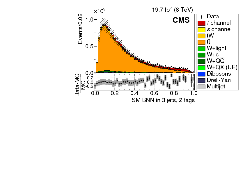Comparison of $\sqrt{s} = 8\TeV$ data and simulation using the SM BNN discriminant in three separate signal regions of two jets with one b-tagged (2 jets, 1 tag) (upper), three jets with one of them b-tagged (3 jets, 1 tag) (middle left), and three jets with two of them b-tagged (3 jets, 2 tags) (middle right), and in \ttbar (4 jets, 2 tags) (lower left) and \wjets (no b-tagged jets) (lower right) background control regions (CR). The lower part of each plot shows the relative difference between the data and the total predicted background. The hatched band corresponds to the total simulation uncertainty. The vertical bars represent the statistical uncertainties.

Comparison of $\sqrt{s} = 8\TeV$ data and simulation using the SM BNN discriminant in three separate signal regions of two jets with one b-tagged (2 jets, 1 tag) (upper), three jets with one of them b-tagged (3 jets, 1 tag) (middle left), and three jets with two of them b-tagged (3 jets, 2 tags) (middle right), and in \ttbar (4 jets, 2 tags) (lower left) and \wjets (no b-tagged jets) (lower right) background control regions (CR). The lower part of each plot shows the relative difference between the data and the total predicted background. The hatched band corresponds to the total simulation uncertainty. The vertical bars represent the statistical uncertainties.

Comparison of $\sqrt{s} = 8\TeV$ data and simulation using the SM BNN discriminant in three separate signal regions of two jets with one b-tagged (2 jets, 1 tag) (upper), three jets with one of them b-tagged (3 jets, 1 tag) (middle left), and three jets with two of them b-tagged (3 jets, 2 tags) (middle right), and in \ttbar (4 jets, 2 tags) (lower left) and \wjets (no b-tagged jets) (lower right) background control regions (CR). The lower part of each plot shows the relative difference between the data and the total predicted background. The hatched band corresponds to the total simulation uncertainty. The vertical bars represent the statistical uncertainties.

The SM BNN discriminant distributions after the statistical analysis and evaluation of all the uncertainties. The lower part of each plot shows the relative difference between the data and the total predicted background. The hatched band corresponds to the total simulation uncertainty. The vertical bars represent the statistical uncertainties. The left (right) plot corresponds to $\sqrt{s}=7$ (8)\TeV.

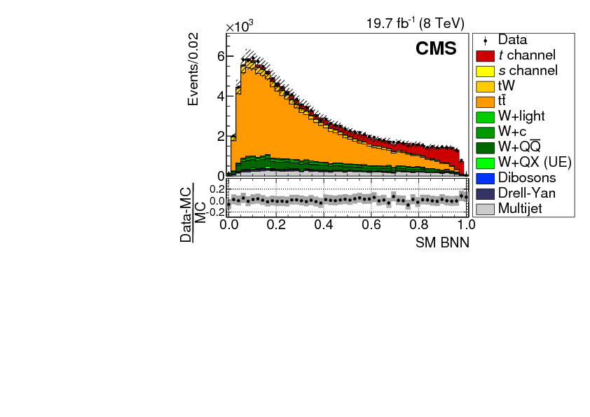The SM BNN discriminant distributions after the statistical analysis and evaluation of all the uncertainties. The lower part of each plot shows the relative difference between the data and the total predicted background. The hatched band corresponds to the total simulation uncertainty. The vertical bars represent the statistical uncertainties. The left (right) plot corresponds to $\sqrt{s}=7$ (8)\TeV.

Distributions of the Wtb BNN discriminants from data (points) and simulation (filled histograms) for the scenarios $(f_{\rm V}^{\rm L}$, $f_{\rm V}^{\rm R})$ (top), $(f_{\rm V}^{\rm L}$, $f_{\rm T}^{\rm L})$ (middle), and $(f_{\rm V}^{\rm L}$, $f_{\rm T}^{\rm R})$ (bottom). The plots on the left (right) correspond to $\sqrt{s}=7$ (8)\TeV. The Wtb BNNs are trained to separate SM left-handed interactions from one of the anomalous interactions. In each plot, the expected distribution with the corresponding anomalous coupling set to 1.0 is shown by the solid curve. The lower part of each plot shows the relative difference between the data and the total predicted background. The hatched band corresponds to the total simulation uncertainty. The vertical bars represent the statistical uncertainties.

Distributions of the Wtb BNN discriminants from data (points) and simulation (filled histograms) for the scenarios $(f_{\rm V}^{\rm L}$, $f_{\rm V}^{\rm R})$ (top), $(f_{\rm V}^{\rm L}$, $f_{\rm T}^{\rm L})$ (middle), and $(f_{\rm V}^{\rm L}$, $f_{\rm T}^{\rm R})$ (bottom). The plots on the left (right) correspond to $\sqrt{s}=7$ (8)\TeV. The Wtb BNNs are trained to separate SM left-handed interactions from one of the anomalous interactions. In each plot, the expected distribution with the corresponding anomalous coupling set to 1.0 is shown by the solid curve. The lower part of each plot shows the relative difference between the data and the total predicted background. The hatched band corresponds to the total simulation uncertainty. The vertical bars represent the statistical uncertainties.

Distributions of the Wtb BNN discriminants from data (points) and simulation (filled histograms) for the scenarios $(f_{\rm V}^{\rm L}$, $f_{\rm V}^{\rm R})$ (top), $(f_{\rm V}^{\rm L}$, $f_{\rm T}^{\rm L})$ (middle), and $(f_{\rm V}^{\rm L}$, $f_{\rm T}^{\rm R})$ (bottom). The plots on the left (right) correspond to $\sqrt{s}=7$ (8)\TeV. The Wtb BNNs are trained to separate SM left-handed interactions from one of the anomalous interactions. In each plot, the expected distribution with the corresponding anomalous coupling set to 1.0 is shown by the solid curve. The lower part of each plot shows the relative difference between the data and the total predicted background. The hatched band corresponds to the total simulation uncertainty. The vertical bars represent the statistical uncertainties.

Distributions of the Wtb BNN discriminants from data (points) and simulation (filled histograms) for the scenarios $(f_{\rm V}^{\rm L}$, $f_{\rm V}^{\rm R})$ (top), $(f_{\rm V}^{\rm L}$, $f_{\rm T}^{\rm L})$ (middle), and $(f_{\rm V}^{\rm L}$, $f_{\rm T}^{\rm R})$ (bottom). The plots on the left (right) correspond to $\sqrt{s}=7$ (8)\TeV. The Wtb BNNs are trained to separate SM left-handed interactions from one of the anomalous interactions. In each plot, the expected distribution with the corresponding anomalous coupling set to 1.0 is shown by the solid curve. The lower part of each plot shows the relative difference between the data and the total predicted background. The hatched band corresponds to the total simulation uncertainty. The vertical bars represent the statistical uncertainties.

Distributions of the Wtb BNN discriminants from data (points) and simulation (filled histograms) for the scenarios $(f_{\rm V}^{\rm L}$, $f_{\rm V}^{\rm R})$ (top), $(f_{\rm V}^{\rm L}$, $f_{\rm T}^{\rm L})$ (middle), and $(f_{\rm V}^{\rm L}$, $f_{\rm T}^{\rm R})$ (bottom). The plots on the left (right) correspond to $\sqrt{s}=7$ (8)\TeV. The Wtb BNNs are trained to separate SM left-handed interactions from one of the anomalous interactions. In each plot, the expected distribution with the corresponding anomalous coupling set to 1.0 is shown by the solid curve. The lower part of each plot shows the relative difference between the data and the total predicted background. The hatched band corresponds to the total simulation uncertainty. The vertical bars represent the statistical uncertainties.

Distributions of the Wtb BNN discriminants from data (points) and simulation (filled histograms) for the scenarios $(f_{\rm V}^{\rm L}$, $f_{\rm V}^{\rm R})$ (top), $(f_{\rm V}^{\rm L}$, $f_{\rm T}^{\rm L})$ (middle), and $(f_{\rm V}^{\rm L}$, $f_{\rm T}^{\rm R})$ (bottom). The plots on the left (right) correspond to $\sqrt{s}=7$ (8)\TeV. The Wtb BNNs are trained to separate SM left-handed interactions from one of the anomalous interactions. In each plot, the expected distribution with the corresponding anomalous coupling set to 1.0 is shown by the solid curve. The lower part of each plot shows the relative difference between the data and the total predicted background. The hatched band corresponds to the total simulation uncertainty. The vertical bars represent the statistical uncertainties.

Combined $\sqrt{s}=7$ and $8\TeV$ observed and expected exclusion limits in the two-dimensional planes $(f_{\rm V}^{\rm L}$, $\lvert f_{\rm V}^{\rm R}\rvert)$ (top-left), $(f_{\rm V}^{\rm L}$, $\lvert f_{\rm T}^{\rm L}\rvert)$ (top-right), and $(f_{\rm V}^{\rm L}$, $f_{\rm T}^{\rm R})$ (bottom) at 68\% and 95\% CL.

Combined $\sqrt{s}=7$ and $8\TeV$ observed and expected exclusion limits in the two-dimensional planes $(f_{\rm V}^{\rm L}$, $\lvert f_{\rm V}^{\rm R}\rvert)$ (top-left), $(f_{\rm V}^{\rm L}$, $\lvert f_{\rm T}^{\rm L}\rvert)$ (top-right), and $(f_{\rm V}^{\rm L}$, $f_{\rm T}^{\rm R})$ (bottom) at 68\% and 95\% CL.

Combined $\sqrt{s}=7$ and $8\TeV$ observed and expected exclusion limits in the two-dimensional planes $(f_{\rm V}^{\rm L}$, $\lvert f_{\rm V}^{\rm R}\rvert)$ (top-left), $(f_{\rm V}^{\rm L}$, $\lvert f_{\rm T}^{\rm L}\rvert)$ (top-right), and $(f_{\rm V}^{\rm L}$, $f_{\rm T}^{\rm R})$ (bottom) at 68\% and 95\% CL.

Combined $\sqrt{s}=7$ and $8\TeV$ results from the three-dimensional variation of the couplings of $f_{\rm V}^{\rm L}$, $f_{\rm T}^{\rm L}$, $f_{\rm T}^{\rm R}$ (left), and $f_{\rm V}^{\rm L}$, $f_{\rm V}^{\rm R}$, $f_{\rm T}^{\rm R}$ (right) in the form of observed and expected exclusion limits at 68\% and 95\% CL in the two-dimension planes $(\lvert f_{\rm T}^{\rm L}\rvert$, $f_{\rm T}^{\rm R})$ (left) and $(\lvert f_{\rm V}^{\rm R}\rvert $, $f_{\rm T}^{\rm R})$ (right).

Combined $\sqrt{s}=7$ and $8\TeV$ results from the three-dimensional variation of the couplings of $f_{\rm V}^{\rm L}$, $f_{\rm T}^{\rm L}$, $f_{\rm T}^{\rm R}$ (left), and $f_{\rm V}^{\rm L}$, $f_{\rm V}^{\rm R}$, $f_{\rm T}^{\rm R}$ (right) in the form of observed and expected exclusion limits at 68\% and 95\% CL in the two-dimension planes $(\lvert f_{\rm T}^{\rm L}\rvert$, $f_{\rm T}^{\rm R})$ (left) and $(\lvert f_{\rm V}^{\rm R}\rvert $, $f_{\rm T}^{\rm R})$ (right).

Representative Feynman diagrams for the FCNC processes.

The FCNC BNN discriminant distributions when the BNN is trained to distinguish $\rm t\to ug$ (upper) or $\rm t\to cg$ (lower) processes as signal from the SM processes as background. The results from data are shown as points and the predicted distributions from the background simulations by the filled histograms. The plots on the left (right) correspond to the $\sqrt{s} = 7$ (8)\TeV data. The solid and dashed lines give the expected distributions for $\rm t\to ug$ and $\rm t\to cg$, respectively, assuming a coupling of $\lvert\kappa_\mathrm{tug}\rvert/\Lambda = 0.04\ (0.06)$ and $\lvert\kappa_\mathrm{tcg}\rvert/\Lambda = 0.08\ (0.12)\TeV^{-1}$ on the left (right) plots. The lower part of each plot shows the relative difference between the data and the total predicted background. The hatched band corresponds to the total simulation uncertainty. The vertical bars represent the statistical uncertainties.

The FCNC BNN discriminant distributions when the BNN is trained to distinguish $\rm t\to ug$ (upper) or $\rm t\to cg$ (lower) processes as signal from the SM processes as background. The results from data are shown as points and the predicted distributions from the background simulations by the filled histograms. The plots on the left (right) correspond to the $\sqrt{s} = 7$ (8)\TeV data. The solid and dashed lines give the expected distributions for $\rm t\to ug$ and $\rm t\to cg$, respectively, assuming a coupling of $\lvert\kappa_\mathrm{tug}\rvert/\Lambda = 0.04\ (0.06)$ and $\lvert\kappa_\mathrm{tcg}\rvert/\Lambda = 0.08\ (0.12)\TeV^{-1}$ on the left (right) plots. The lower part of each plot shows the relative difference between the data and the total predicted background. The hatched band corresponds to the total simulation uncertainty. The vertical bars represent the statistical uncertainties.

The FCNC BNN discriminant distributions when the BNN is trained to distinguish $\rm t\to ug$ (upper) or $\rm t\to cg$ (lower) processes as signal from the SM processes as background. The results from data are shown as points and the predicted distributions from the background simulations by the filled histograms. The plots on the left (right) correspond to the $\sqrt{s} = 7$ (8)\TeV data. The solid and dashed lines give the expected distributions for $\rm t\to ug$ and $\rm t\to cg$, respectively, assuming a coupling of $\lvert\kappa_\mathrm{tug}\rvert/\Lambda = 0.04\ (0.06)$ and $\lvert\kappa_\mathrm{tcg}\rvert/\Lambda = 0.08\ (0.12)\TeV^{-1}$ on the left (right) plots. The lower part of each plot shows the relative difference between the data and the total predicted background. The hatched band corresponds to the total simulation uncertainty. The vertical bars represent the statistical uncertainties.

The FCNC BNN discriminant distributions when the BNN is trained to distinguish $\rm t\to ug$ (upper) or $\rm t\to cg$ (lower) processes as signal from the SM processes as background. The results from data are shown as points and the predicted distributions from the background simulations by the filled histograms. The plots on the left (right) correspond to the $\sqrt{s} = 7$ (8)\TeV data. The solid and dashed lines give the expected distributions for $\rm t\to ug$ and $\rm t\to cg$, respectively, assuming a coupling of $\lvert\kappa_\mathrm{tug}\rvert/\Lambda = 0.04\ (0.06)$ and $\lvert\kappa_\mathrm{tcg}\rvert/\Lambda = 0.08\ (0.12)\TeV^{-1}$ on the left (right) plots. The lower part of each plot shows the relative difference between the data and the total predicted background. The hatched band corresponds to the total simulation uncertainty. The vertical bars represent the statistical uncertainties.

Combined $\sqrt{s}$ = 7 and 8\TeV observed and expected limits for the 68\% and 95\% CL on the $\lvert\kappa_\mathrm{tug}\rvert/\Lambda$ and $\lvert\kappa_\mathrm{tcg}\rvert/\Lambda$ couplings.