CERN Accelerating science

 
Large Primordial Trispectra in General Single Field Inflation - Chen, Xingang et al - arXiv:0905.3494MIT-CTP-4039CAS-KITPC-ITP-111CERN-PH-TH-2009-064MAD-TH-09-04
 
Two diagrams that contribute to the large trispectra.
This figure illustrates the tetrahedron weconsider.
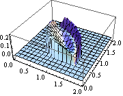
In this group of figures, we consider the equilateral limit $k_1=k_2=k_3=k_4$, and plot $T_{s1}$, $T_{s2}$, $T_{s3}$, $T_{c1}$, $T_{loc1}$ and $T_{loc2}$, respectively, as functions of $k_{12}/k_1$ and $k_{14}/k_1$. Note that $T_{loc1}$ blows up when $k_{12}\ll k_1$ and $k_{14} \ll k_1$. $T_{loc1}$ also blows up in the other boundary, because this boundary corresponds to $k_{13}\ll k_1$. So $T_{loc1}$ is distinguishable from all other shapes in this limit. We also notethat $T_{c1}$ and $T_{loc2}$ are both independent of $k_{12}$ and $k_{14}$.
In this group of figures, we consider the folded limit $k_{12}=0$, and plot $T_{s1}$, $T_{s2}$, $T_{s3}$, $T_{c1}$ and $T_{loc2}$, respectively, as functions of $k_{14}/k_1$ and $k_{4}/k_1$. $T_{loc1}$ blows up in this limit. Note that when $k_4\rightarrow 0$, allshape functions except $T_{loc1}$ and $T_{loc2}$ vanish.
In this group of figures, we consider the specialized planar limit with $k_1=k_3=k_{14}$, and plot $T_{s1}$, $T_{s2}$, $T_{s3}$, $T_{c1}$, $T_{loc1}$ and $T_{loc2}$, respectively, as functions of $k_{2}/k_1$ and $k_{4}/k_1$. Again, in the $k_2\rightarrow 0$ or $k_4\rightarrow 0$ limit, our shape functions vanish as $\CO(k_2^2)$ and $\CO(k_4^2)$ respectively. This is different from that of the local shape. $T_{loc1}$ blows up when $k_2 \rightarrow k_4$. This is because inthis limit, $k_{13}\rightarrow 0$.
In this group of figures, we look at the shapes near the double squeezed limit: we consider the case where ${k}_3={k}_4=k_{12}$ and the tetrahedron is a planar quadrangle. We plot $T_{s1}/(\prod_{i=1}^4 k_i)$, $T_{s2}/(\prod k_i)$, $T_{s3}/(\prod k_i)$, $T_{c1}/(\prod k_i)$, $T_{loc1}/(\prod k_i)$ and $T_{loc2}/(\prod k_i)$, respectively, as functions of $k_{12}/k_1$ and $k_{14}/k_1$. Note that, taking the double-squeezed limit $k_4\rightarrow 0$, the scalar-exchange contributions $T_{s1}/(\prod k_i)$, $T_{s2}/(\prod k_i)$, $T_{s3}/(\prod k_i)$ are nonzero and finite, and the contact-interaction $T_{c1}/(\prod k_i)$ vanishes. As a comparison, the local form terms $T_{loc1}/(\prod k_i)$ and $T_{loc2}/(\prod k_i)$ blow up. The different behaviors in the folded and squeezedlimit can also been seen from this figure (see the main text for details).
In this group of figures, we plot the $\tilde T_{c1}/{\rm Re}(C_-)$ (the left column) and $\tilde T_{s1}/{\rm Re}(C_-)$ (the right column) in the equilateral limit, specialized planar limit, and near double squeezed limit (we plot $\tilde T_{c1}/[{\rm Re}(C_-)\Pi_i k_i]$ and $\tilde T_{s1}/[{\rm Re}(C_-)\Pi_i k_i]$ in near double squeezed limit) respectively. Note that, in order to show clearly the locations of the divergence, in some figures we have taken thecutoffs of the z-axes to be extremely large.
The quadrangles in black and blue represents the solution (\ref{planark2}) with minus and plus sign respectively. The term with plus sign corresponds to the blue quadrangle, and can be transformed into another quadrangle corresponding to the minus solution by a symmetry discussed in Eq.\eqref{symeq}.
In the six rows, we plot $T_{s1}$, $T_{s2}$, $T_{s3}$, $T_{c1}$, $T_{loc1}$ and $T_{loc2}$ respectively as functions of $k_{12}/k_1$ and $k_{14}/k_1$ in the planar limit. Within each row, the momenta configuration is $(k_3/k_1,k_4/k_1)=\{(0.6,0.6),(0.6,1.0),(1.0,0.6),(1.0,1.0)\}$ respectively in the four columns, as given in \eqref{groupfigk}.