CERN Accelerating science

Example Feynman diagrams for the signal processes.

Example Feynman diagrams for the signal processes.

Example Feynman diagrams for the signal processes.

Signal efficiency as a function of the mass \mPhi after triple \PQb tag selection for 2017 SL (squares), 2017 FH (triangles), and 2018 FH (circles) channels.

Simulated signal yields normalized to unit area for three representative values of the Higgs boson mass \mPhi in the 2017 SL (upper left), 2017 FH (upper right), and 2018 FH (lower) channels. The solid curves show the signal parameterisations by double-sided Crystal Ball probability density functions.

Simulated signal yields normalized to unit area for three representative values of the Higgs boson mass \mPhi in the 2017 SL (upper left), 2017 FH (upper right), and 2018 FH (lower) channels. The solid curves show the signal parameterisations by double-sided Crystal Ball probability density functions.

Simulated signal yields normalized to unit area for three representative values of the Higgs boson mass \mPhi in the 2017 SL (upper left), 2017 FH (upper right), and 2018 FH (lower) channels. The solid curves show the signal parameterisations by double-sided Crystal Ball probability density functions.

Invariant mass distributions of the three fit ranges in the \PQb tag veto CR for the 2017 SL channel, overlaid with the fitted functions. The distributions are fitted in the \mjj ranges of 120--300\GeV (upper left), 180--460\GeV (upper right), and 240--800\GeV (lower). The $\chi^2$ and the corresponding p-value obtained from the goodness-of-fit test are displayed on each plot. The lower panels show the difference between the data and the fitted function, divided by the estimated statistical uncertainty for each bin. Good agreement between the fitted functions and the data is achieved.

Invariant mass distributions of the three fit ranges in the \PQb tag veto CR for the 2017 SL channel, overlaid with the fitted functions. The distributions are fitted in the \mjj ranges of 120--300\GeV (upper left), 180--460\GeV (upper right), and 240--800\GeV (lower). The $\chi^2$ and the corresponding p-value obtained from the goodness-of-fit test are displayed on each plot. The lower panels show the difference between the data and the fitted function, divided by the estimated statistical uncertainty for each bin. Good agreement between the fitted functions and the data is achieved.

Invariant mass distributions of the three fit ranges in the \PQb tag veto CR for the 2017 SL channel, overlaid with the fitted functions. The distributions are fitted in the \mjj ranges of 120--300\GeV (upper left), 180--460\GeV (upper right), and 240--800\GeV (lower). The $\chi^2$ and the corresponding p-value obtained from the goodness-of-fit test are displayed on each plot. The lower panels show the difference between the data and the fitted function, divided by the estimated statistical uncertainty for each bin. Good agreement between the fitted functions and the data is achieved.

Invariant mass distributions of the four fit ranges in the \PQb tag veto CR for the 2017 FH channel, overlaid with the fitted functions. The distributions are fitted in the \mjj ranges of 240--560\GeV (upper left), 280--800\GeV (upper right), 400--1300\GeV (lower left), and 600--2000\GeV (lower right). The $\chi^2$ goodness-of-fit test and corresponding p-value are indicated in each plot. The lower panels show the difference between the data and the fitted function, divided by the estimated statistical uncertainty for each bin. Good agreement between the fitted functions and the data is achieved.

Invariant mass distributions of the four fit ranges in the \PQb tag veto CR for the 2017 FH channel, overlaid with the fitted functions. The distributions are fitted in the \mjj ranges of 240--560\GeV (upper left), 280--800\GeV (upper right), 400--1300\GeV (lower left), and 600--2000\GeV (lower right). The $\chi^2$ goodness-of-fit test and corresponding p-value are indicated in each plot. The lower panels show the difference between the data and the fitted function, divided by the estimated statistical uncertainty for each bin. Good agreement between the fitted functions and the data is achieved.

Invariant mass distributions of the four fit ranges in the \PQb tag veto CR for the 2017 FH channel, overlaid with the fitted functions. The distributions are fitted in the \mjj ranges of 240--560\GeV (upper left), 280--800\GeV (upper right), 400--1300\GeV (lower left), and 600--2000\GeV (lower right). The $\chi^2$ goodness-of-fit test and corresponding p-value are indicated in each plot. The lower panels show the difference between the data and the fitted function, divided by the estimated statistical uncertainty for each bin. Good agreement between the fitted functions and the data is achieved.

Invariant mass distributions of the four fit ranges in the \PQb tag veto CR for the 2017 FH channel, overlaid with the fitted functions. The distributions are fitted in the \mjj ranges of 240--560\GeV (upper left), 280--800\GeV (upper right), 400--1300\GeV (lower left), and 600--2000\GeV (lower right). The $\chi^2$ goodness-of-fit test and corresponding p-value are indicated in each plot. The lower panels show the difference between the data and the fitted function, divided by the estimated statistical uncertainty for each bin. Good agreement between the fitted functions and the data is achieved.

Invariant mass distributions of the four fit ranges in the \PQb tag veto CR for the 2018 FH channel, overlaid with the fitted functions. The distributions are fitted in the \mjj ranges of 270--560\GeV (upper left), 320--800\GeV (upper right), 390--1270\GeV (lower left), and 500--2000\GeV (lower right). The $\chi^2$ goodness-of-fit test and corresponding p-value are indicated in each plot. The lower panels show the difference between the data and the fitted function, divided by the estimated statistical uncertainty for each bin. Good agreement between the fitted functions and the data is achieved.

Invariant mass distributions of the four fit ranges in the \PQb tag veto CR for the 2018 FH channel, overlaid with the fitted functions. The distributions are fitted in the \mjj ranges of 270--560\GeV (upper left), 320--800\GeV (upper right), 390--1270\GeV (lower left), and 500--2000\GeV (lower right). The $\chi^2$ goodness-of-fit test and corresponding p-value are indicated in each plot. The lower panels show the difference between the data and the fitted function, divided by the estimated statistical uncertainty for each bin. Good agreement between the fitted functions and the data is achieved.

Invariant mass distributions of the four fit ranges in the \PQb tag veto CR for the 2018 FH channel, overlaid with the fitted functions. The distributions are fitted in the \mjj ranges of 270--560\GeV (upper left), 320--800\GeV (upper right), 390--1270\GeV (lower left), and 500--2000\GeV (lower right). The $\chi^2$ goodness-of-fit test and corresponding p-value are indicated in each plot. The lower panels show the difference between the data and the fitted function, divided by the estimated statistical uncertainty for each bin. Good agreement between the fitted functions and the data is achieved.

Invariant mass distributions of the four fit ranges in the \PQb tag veto CR for the 2018 FH channel, overlaid with the fitted functions. The distributions are fitted in the \mjj ranges of 270--560\GeV (upper left), 320--800\GeV (upper right), 390--1270\GeV (lower left), and 500--2000\GeV (lower right). The $\chi^2$ goodness-of-fit test and corresponding p-value are indicated in each plot. The lower panels show the difference between the data and the fitted function, divided by the estimated statistical uncertainty for each bin. Good agreement between the fitted functions and the data is achieved.

Background-only fits to the \mjj~distribution in each fit range of the 2017 analysis in the SL category, shown together with ${\pm}1\sigma$ and ${\pm}2\sigma$ uncertainty bands extracted from the fit in the upper panels. The lower panels show the difference between data and fitted background, divided by the statistical uncertainty of the latter. The distributions are fitted in the \mjj ranges of 120--300\GeV (upper left), 180--460\GeV (upper right), and 240--800\GeV (lower).

Background-only fits to the \mjj~distribution in each fit range of the 2017 analysis in the SL category, shown together with ${\pm}1\sigma$ and ${\pm}2\sigma$ uncertainty bands extracted from the fit in the upper panels. The lower panels show the difference between data and fitted background, divided by the statistical uncertainty of the latter. The distributions are fitted in the \mjj ranges of 120--300\GeV (upper left), 180--460\GeV (upper right), and 240--800\GeV (lower).

Background-only fits to the \mjj~distribution in each fit range of the 2017 analysis in the SL category, shown together with ${\pm}1\sigma$ and ${\pm}2\sigma$ uncertainty bands extracted from the fit in the upper panels. The lower panels show the difference between data and fitted background, divided by the statistical uncertainty of the latter. The distributions are fitted in the \mjj ranges of 120--300\GeV (upper left), 180--460\GeV (upper right), and 240--800\GeV (lower).

Background-only fits to the \mjj~distribution in each fit range of the 2017 analysis in the FH category, shown together with ${\pm}1\sigma$ and ${\pm}2\sigma$ uncertainty bands extracted from the fit in the upper panels. The lower panels show the difference between data and fitted background, divided by the statistical uncertainty of the latter. The distributions are fitted in the \mjj ranges of 240--560\GeV (upper left), 280--800\GeV (upper right), 400--1300\GeV (lower left), and 600--2000\GeV (lower right).

Background-only fits to the \mjj~distribution in each fit range of the 2017 analysis in the FH category, shown together with ${\pm}1\sigma$ and ${\pm}2\sigma$ uncertainty bands extracted from the fit in the upper panels. The lower panels show the difference between data and fitted background, divided by the statistical uncertainty of the latter. The distributions are fitted in the \mjj ranges of 240--560\GeV (upper left), 280--800\GeV (upper right), 400--1300\GeV (lower left), and 600--2000\GeV (lower right).

Background-only fits to the \mjj~distribution in each fit range of the 2017 analysis in the FH category, shown together with ${\pm}1\sigma$ and ${\pm}2\sigma$ uncertainty bands extracted from the fit in the upper panels. The lower panels show the difference between data and fitted background, divided by the statistical uncertainty of the latter. The distributions are fitted in the \mjj ranges of 240--560\GeV (upper left), 280--800\GeV (upper right), 400--1300\GeV (lower left), and 600--2000\GeV (lower right).

Background-only fits to the \mjj~distribution in each fit range of the 2017 analysis in the FH category, shown together with ${\pm}1\sigma$ and ${\pm}2\sigma$ uncertainty bands extracted from the fit in the upper panels. The lower panels show the difference between data and fitted background, divided by the statistical uncertainty of the latter. The distributions are fitted in the \mjj ranges of 240--560\GeV (upper left), 280--800\GeV (upper right), 400--1300\GeV (lower left), and 600--2000\GeV (lower right).

Background-only fits to the \mjj~distribution in each fit range of the 2018 analysis in the FH category, shown together with ${\pm}1\sigma$ and ${\pm}2\sigma$ uncertainty bands extracted from the fit in the upper panels. The lower panels show the difference between data and fitted background, divided by the statistical uncertainty of the latter. The distributions are fitted in the \mjj ranges of 270--560\GeV (upper left), 320--800\GeV (upper right), 390--1270\GeV (lower left), and 500--2000\GeV (lower right).

Background-only fits to the \mjj~distribution in each fit range of the 2018 analysis in the FH category, shown together with ${\pm}1\sigma$ and ${\pm}2\sigma$ uncertainty bands extracted from the fit in the upper panels. The lower panels show the difference between data and fitted background, divided by the statistical uncertainty of the latter. The distributions are fitted in the \mjj ranges of 270--560\GeV (upper left), 320--800\GeV (upper right), 390--1270\GeV (lower left), and 500--2000\GeV (lower right).

Background-only fits to the \mjj~distribution in each fit range of the 2018 analysis in the FH category, shown together with ${\pm}1\sigma$ and ${\pm}2\sigma$ uncertainty bands extracted from the fit in the upper panels. The lower panels show the difference between data and fitted background, divided by the statistical uncertainty of the latter. The distributions are fitted in the \mjj ranges of 270--560\GeV (upper left), 320--800\GeV (upper right), 390--1270\GeV (lower left), and 500--2000\GeV (lower right).

Background-only fits to the \mjj~distribution in each fit range of the 2018 analysis in the FH category, shown together with ${\pm}1\sigma$ and ${\pm}2\sigma$ uncertainty bands extracted from the fit in the upper panels. The lower panels show the difference between data and fitted background, divided by the statistical uncertainty of the latter. The distributions are fitted in the \mjj ranges of 270--560\GeV (upper left), 320--800\GeV (upper right), 390--1270\GeV (lower left), and 500--2000\GeV (lower right).

Expected and observed upper limits for the \PQb-quark-associated Higgs boson production cross section times branching fraction of the decay into a \PQb quark pair at 95\% CL as functions of \mPhi for the 2017 SL category. The vertical dashed lines indicate the boundaries of usage of the different fit ranges, as reflected in the rightmost column of Table~\ref{tab:massrangedefs}.

Expected and observed upper limits for the \PQb-quark-associated Higgs boson production cross section times branching fraction of the decay into a \PQb quark pair at 95\% CL as functions of \mPhi for the 2017 FH category. The vertical dashed lines indicate the boundaries of usage of the different fit ranges, as reflected in the rightmost column of Table~\ref{tab:massrangedefs}.

Expected and observed upper limits for the \PQb-quark-associated Higgs boson production cross section times branching fraction of the decay into a \PQb quark pair at 95\% CL as functions of \mPhi for the 2018 FH category. The vertical dashed lines indicate the boundaries of usage of the different fit ranges, as reflected in the rightmost column of Table~\ref{tab:massrangedefs}.

Expected and observed upper limits for the \PQb-quark-associated Higgs boson production cross section times branching fraction of the decay into a \PQb quark pair at 95\% CL as functions of \mPhi, corresponding to the combination with the 2016 data. The vertical dashed line separates the mass range where only the 2017 SL category contributes on its left, from the region where also the 2017 FH and 2018 FH categories contribute on its right. The expected limits from the 2017~SL, 2017~FH, and 2018~FH datasets as well as from the previously published result based on the 2016 dataset are also shown as colored lines.

Interpretation in the \mhmass scenario of the MSSM: observed and expected upper limits at 95\% \CL on the parameter \tanb as functions of the mass \mA of the \CP-odd Higgs boson. The higgsino mass parameter has been set to $\mu = +1\TeV$. The hashed area indicates the parameter region in which the mass of the lightest MSSM Higgs boson does not coincide with 125\GeV within a margin of 3\GeV.

Interpretation in the \mhmass scenario of the MSSM: observed and expected upper limits at 95\% \CL on the parameter \tanb as functions of the mass \mA of the \CP-odd Higgs boson. The higgsino mass parameter has been set to $\mu = -1\TeV$ (upper left), $\mu = -2\TeV$ (upper right), and $\mu = -3\TeV$ (lower). The hashed area indicates the parameter region in which the mass of the lightest MSSM Higgs boson does not coincide with 125\GeV within a margin of 3\GeV.

Interpretation in the \mhmass scenario of the MSSM: observed and expected upper limits at 95\% \CL on the parameter \tanb as functions of the mass \mA of the \CP-odd Higgs boson. The higgsino mass parameter has been set to $\mu = -1\TeV$ (upper left), $\mu = -2\TeV$ (upper right), and $\mu = -3\TeV$ (lower). The hashed area indicates the parameter region in which the mass of the lightest MSSM Higgs boson does not coincide with 125\GeV within a margin of 3\GeV.

Interpretation in the \mhmass scenario of the MSSM: observed and expected upper limits at 95\% \CL on the parameter \tanb as functions of the mass \mA of the \CP-odd Higgs boson. The higgsino mass parameter has been set to $\mu = -1\TeV$ (upper left), $\mu = -2\TeV$ (upper right), and $\mu = -3\TeV$ (lower). The hashed area indicates the parameter region in which the mass of the lightest MSSM Higgs boson does not coincide with 125\GeV within a margin of 3\GeV.

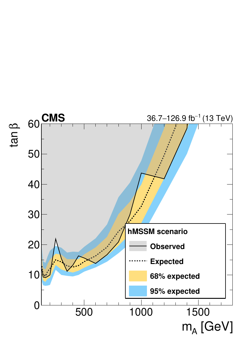
Interpretation in the \mhmodp (left) and hMSSM (right) scenarios of the MSSM: observed and expected upper limits at 95\% \CL on the parameter \tanb as functions of the mass \mA of the \CP-odd Higgs boson. In the left plot, the hashed area indicates the parameter region in which the mass of the lightest MSSM Higgs boson does not coincide with 125\GeV within a margin of 3\GeV.

Interpretation in the \mhmodp (left) and hMSSM (right) scenarios of the MSSM: observed and expected upper limits at 95\% \CL on the parameter \tanb as functions of the mass \mA of the \CP-odd Higgs boson. In the left plot, the hashed area indicates the parameter region in which the mass of the lightest MSSM Higgs boson does not coincide with 125\GeV within a margin of 3\GeV.

Interpretation in 2HDM scenarios: observed and expected upper limits at 95\% \CL on the parameter \tanb as a function of \mAH for $\cosba=0.1$ (left), and as functions of \cosba for masses of $\mA = \mH = 300\GeV$ (right), for the 2HDM \typetwo scenario (upper), and the 2HDM \flipped scenario (lower).

Interpretation in 2HDM scenarios: observed and expected upper limits at 95\% \CL on the parameter \tanb as a function of \mAH for $\cosba=0.1$ (left), and as functions of \cosba for masses of $\mA = \mH = 300\GeV$ (right), for the 2HDM \typetwo scenario (upper), and the 2HDM \flipped scenario (lower).

Interpretation in 2HDM scenarios: observed and expected upper limits at 95\% \CL on the parameter \tanb as a function of \mAH for $\cosba=0.1$ (left), and as functions of \cosba for masses of $\mA = \mH = 300\GeV$ (right), for the 2HDM \typetwo scenario (upper), and the 2HDM \flipped scenario (lower).

Interpretation in 2HDM scenarios: observed and expected upper limits at 95\% \CL on the parameter \tanb as a function of \mAH for $\cosba=0.1$ (left), and as functions of \cosba for masses of $\mA = \mH = 300\GeV$ (right), for the 2HDM \typetwo scenario (upper), and the 2HDM \flipped scenario (lower).

Interpretation in the 2HDM flipped scenario: observed and expected upper limits at 95\% \CL on the parameter \tanb as functions of \cosba for masses of $\mA = \mH = 140$, 600, 900, and 1200\GeV.

Interpretation in the 2HDM flipped scenario: observed and expected upper limits at 95\% \CL on the parameter \tanb as functions of \cosba for masses of $\mA = \mH = 140$, 600, 900, and 1200\GeV.

Interpretation in the 2HDM flipped scenario: observed and expected upper limits at 95\% \CL on the parameter \tanb as functions of \cosba for masses of $\mA = \mH = 140$, 600, 900, and 1200\GeV.

Interpretation in the 2HDM flipped scenario: observed and expected upper limits at 95\% \CL on the parameter \tanb as functions of \cosba for masses of $\mA = \mH = 140$, 600, 900, and 1200\GeV.