CERN Accelerating science

 
The tree-level (left) and penguin (right) Feynman diagrams for the decays \bdjpsiks and \bsjpsiks.
The signal efficiency as a function of the decay time for the \bdjpsiks (upper) and \bsjpsiks (lower) decays from simulation for each of the three data-taking years. The vertical bars indicate the statistical uncertainty, and the horizontal bars give bin widths. The curves show the fit results.
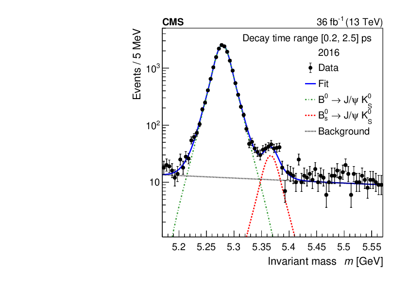
Distributions of the \jpsiks invariant mass (left) and proper decay time (right) from data (points) and the results from the 2D UML fit projections (lines) for the 2016--2018 data set. The vertical bars on the data points indicate the statistical uncertainty. The solid, dotted-dashed, dashed, and dotted lines show the total fit, \bd control channel, \bs signal, and background contributions, respectively.
The proper decay time distribution from data (points) for events in the \bs signal region with \jpsiks invariant mass in the range 5.34--5.42\GeV and the results from the 2D UML fit projections (lines) for the 2016--2018 data set. The vertical bars on the data points indicate the statistical uncertainty. The dashed, dotted-dashed, dotted, and solid lines show the \bs signal, \bd control channel, background, and total fit contributions, respectively.
Distributions of the \jpsiks invariant mass (upper) and decay time (lower) from data (points), along with the projections from the 2D UML fit for each year of data taking. The vertical bars on the data points indicate the statistical uncertainty. The dashed, dotted-dashed, dotted, and solid lines represent the signal, control channel, background, and total fit contributions, respectively.
The decay time distribution for events with \jpsiks invariant mass in the range $5.17 < m < 5.22$ (upper), $5.22 < m < 5.34$ (center), and $5.42 < m < 5.57$ (lower)\GeV and the fit results for the 2016 (left), 2017 (middle), and 2018 (right) data-taking years.
The invariant mass distribution for events with \jpsiks decay time in the range $0.2 < t < 2.5$ (upper), $2.5 < t < 3.5$ (center), and $3.5 < t < 10.0$ (lower)\ps and the fit results for the 2016 (left), 2017 (middle), and 2018 (right) data-taking years.