CERN Accelerating science

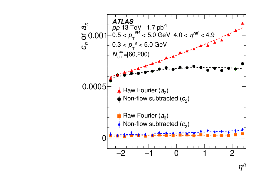Coefficients $a_n$ and $c_n$ in high-multiplicity 13~\TeV\ \pp events for $n = 2, 3$ as a function of track pseudorapidity $\eta^a$. The $c_n$ values are obtained from the template fitting method. The dashed lines represent a fit to a quadratic function in $\eta^a$ for each set of coefficients. The pseudorapidity gap between the cluster and track pair is largest for negative $\eta^a$ and decreases moving to positive $\eta^a$. Only statistical uncertainties are shown.

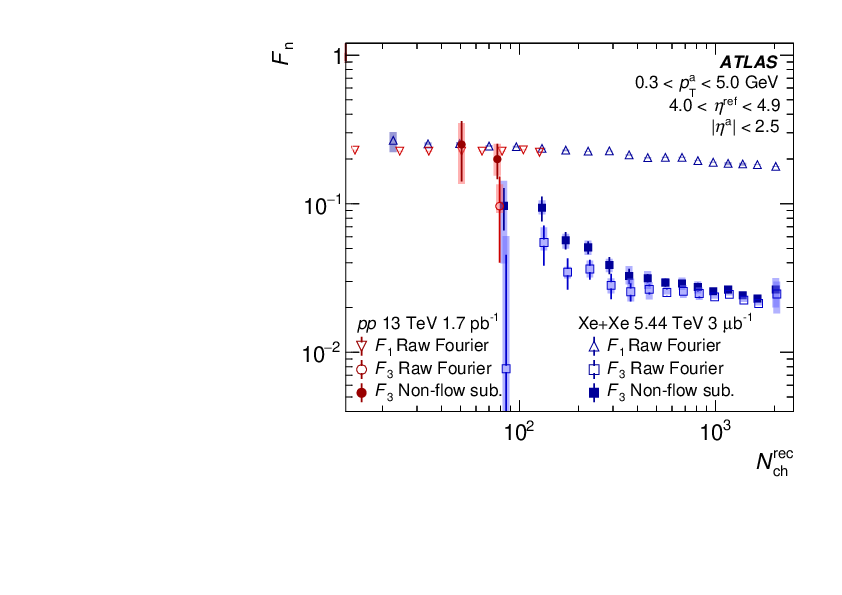
Longitudinal decorrelation parameters $F_n$ for 13~\TeV\ \pp (red) and 5.44~\TeV\ \xexe (blue) for $n=2$ (left) and $n=1,3$ (right) as a function of \Nrec. The parameters are reported after the application of the NFS to the correlation function (solid markers), and those derived from fits to the raw Fourier coefficients (open markers). The statistical (systematic) uncertainties are drawn as vertical lines (shaded boxes). Points with errors exceeding 0.15 are not shown.

Longitudinal decorrelation parameters $F_n$ for 13~\TeV\ \pp (red) and 5.44~\TeV\ \xexe (blue) for $n=2$ (left) and $n=1,3$ (right) as a function of \Nrec. The parameters are reported after the application of the NFS to the correlation function (solid markers), and those derived from fits to the raw Fourier coefficients (open markers). The statistical (systematic) uncertainties are drawn as vertical lines (shaded boxes). Points with errors exceeding 0.15 are not shown.

Comparison of \textsc{AMPT} theory calculations to the 13~\TeV\ \pp (left) and 5.44~\TeV\ \xexe (right) results. In data, the non-flow subtracted $F_n$ values are shown as a function of \Nrec. The statistical (systematic) uncertainties are drawn as vertical lines (shaded bands).

Comparison of \textsc{AMPT} theory calculations to the 13~\TeV\ \pp (left) and 5.44~\TeV\ \xexe (right) results. In data, the non-flow subtracted $F_n$ values are shown as a function of \Nrec. The statistical (systematic) uncertainties are drawn as vertical lines (shaded bands).

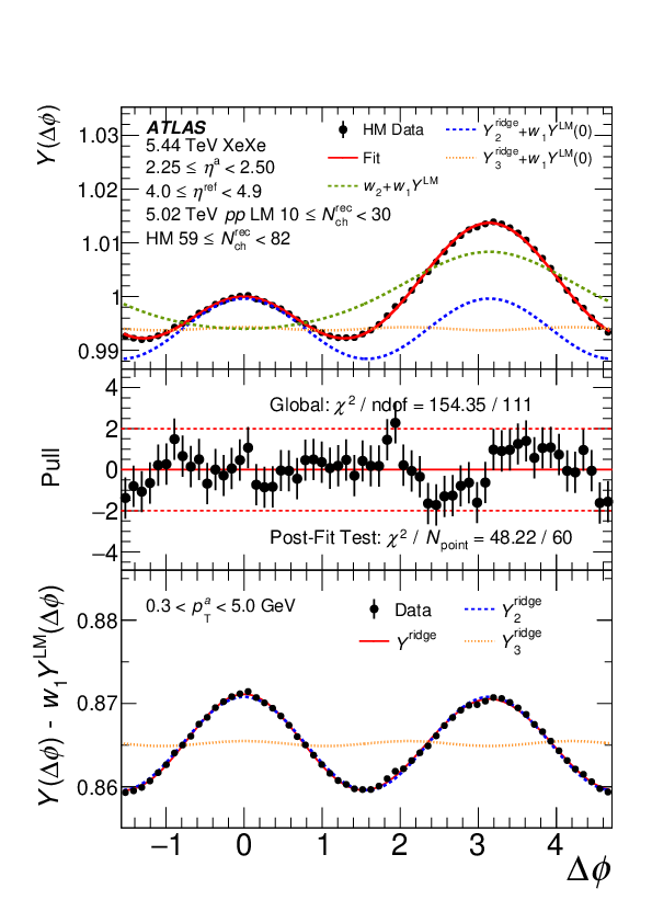
Selected example 2PC template fit results for two $\eta^a$ intervals in 13~\TeV \pp collisions (left) and 5.44~\TeV \xexe collisions (right). In the top panels, the solid red line shows the total fit to the HM data, shown in black markers. The dashed green line shows the scaled LM reference correlation plus pedestal, while the dashed blue and dotted yellow lines indicate the two flow contributions to the fit, $Y_2^\mathrm{ridge} = w_2[1 + 2c_{2}\cos(2\Delta\phi)]$ and $Y_3^\mathrm{ridge} = w_2 [1 + 2c_{3}\cos(3\Delta\phi)]$, shifted upwards by $w_1 Y^\mathrm{LM}(0)$ for visibility. The middle panels show the pull distribution for the template fits. The global $\chi^2$/ndf is calculated from the simultaneous fit to the HM and LM correlations. The post-fit $\chi^2$/$N_{\mathrm{point}}$ is calculated from the pull distribution in the panel. The bottom panels show the same set of data and fit components, where the scaled LM distribution was subtracted from each to better isolate the modulation.

Selected example 2PC template fit results for two $\eta^a$ intervals in 13~\TeV \pp collisions (left) and 5.44~\TeV \xexe collisions (right). In the top panels, the solid red line shows the total fit to the HM data, shown in black markers. The dashed green line shows the scaled LM reference correlation plus pedestal, while the dashed blue and dotted yellow lines indicate the two flow contributions to the fit, $Y_2^\mathrm{ridge} = w_2[1 + 2c_{2}\cos(2\Delta\phi)]$ and $Y_3^\mathrm{ridge} = w_2 [1 + 2c_{3}\cos(3\Delta\phi)]$, shifted upwards by $w_1 Y^\mathrm{LM}(0)$ for visibility. The middle panels show the pull distribution for the template fits. The global $\chi^2$/ndf is calculated from the simultaneous fit to the HM and LM correlations. The post-fit $\chi^2$/$N_{\mathrm{point}}$ is calculated from the pull distribution in the panel. The bottom panels show the same set of data and fit components, where the scaled LM distribution was subtracted from each to better isolate the modulation.

Selected example 2PC template fit results for two $\eta^a$ intervals in 13~\TeV \pp collisions (left) and 5.44~\TeV \xexe collisions (right). In the top panels, the solid red line shows the total fit to the HM data, shown in black markers. The dashed green line shows the scaled LM reference correlation plus pedestal, while the dashed blue and dotted yellow lines indicate the two flow contributions to the fit, $Y_2^\mathrm{ridge} = w_2[1 + 2c_{2}\cos(2\Delta\phi)]$ and $Y_3^\mathrm{ridge} = w_2 [1 + 2c_{3}\cos(3\Delta\phi)]$, shifted upwards by $w_1 Y^\mathrm{LM}(0)$ for visibility. The middle panels show the pull distribution for the template fits. The global $\chi^2$/ndf is calculated from the simultaneous fit to the HM and LM correlations. The post-fit $\chi^2$/$N_{\mathrm{point}}$ is calculated from the pull distribution in the panel. The bottom panels show the same set of data and fit components, where the scaled LM distribution was subtracted from each to better isolate the modulation.

Selected example 2PC template fit results for two $\eta^a$ intervals in 13~\TeV \pp collisions (left) and 5.44~\TeV \xexe collisions (right). In the top panels, the solid red line shows the total fit to the HM data, shown in black markers. The dashed green line shows the scaled LM reference correlation plus pedestal, while the dashed blue and dotted yellow lines indicate the two flow contributions to the fit, $Y_2^\mathrm{ridge} = w_2[1 + 2c_{2}\cos(2\Delta\phi)]$ and $Y_3^\mathrm{ridge} = w_2 [1 + 2c_{3}\cos(3\Delta\phi)]$, shifted upwards by $w_1 Y^\mathrm{LM}(0)$ for visibility. The middle panels show the pull distribution for the template fits. The global $\chi^2$/ndf is calculated from the simultaneous fit to the HM and LM correlations. The post-fit $\chi^2$/$N_{\mathrm{point}}$ is calculated from the pull distribution in the panel. The bottom panels show the same set of data and fit components, where the scaled LM distribution was subtracted from each to better isolate the modulation.

Coefficients $a_n$ and $c_n$ in low-multiplicity (high-multiplicity) 5.44~\TeV\ \xexe events are shown in the left (right) panel, for $n = 2, 3$ as a function of track pseudorapidity $\eta^a$. The $c_n$ values are obtained from the template fitting method. The dashed lines represent a fit to a quadratic function in $\eta^a$ for each set of coefficients. The pseudorapidity gap between the tower and track pair is largest for negative $\eta^a$ and decreases moving to positive $\eta^a$. Only the statistical uncertainties are shown.

Coefficients $a_n$ and $c_n$ in low-multiplicity (high-multiplicity) 5.44~\TeV\ \xexe events are shown in the left (right) panel, for $n = 2, 3$ as a function of track pseudorapidity $\eta^a$. The $c_n$ values are obtained from the template fitting method. The dashed lines represent a fit to a quadratic function in $\eta^a$ for each set of coefficients. The pseudorapidity gap between the tower and track pair is largest for negative $\eta^a$ and decreases moving to positive $\eta^a$. Only the statistical uncertainties are shown.