CERN Accelerating science

 
Hypothetical Feynman diagrams of $\Bds \rightarrow \proton \ell^{-}$ mediated by a hypothetical $Y$ boson.
-
Expected distribution of the MLP response for \BdsTopmu decays as obtained from the \BdToKpi control channel, for (left) Run 1 and (right) Run 2 data. The total (statistical and systematic combined) uncertainty is shown as a light grey band, and the thickness of each horizontal line at the centre indicates the statistical uncertainty. Each interval is normalised to its width.
Hypothetical Feynman diagrams of $\Bds \rightarrow \proton \ell^{-}$ and $\antiproton\ell^{+}$ mediated by a hypothetical $Y$ boson.
Mass distribution of \BdToKpi candidates in data for (left) Run 1 and (right) Run 2. The results of the invariant mass fits are superimposed.
Comparison of the distributions of the \Bd vertex fit \chisq ($\chi^2_{\mathrm{fit}}(B^0)$) and the minimum \chisqip of the two tracks in the final state ($\mathrm{Min}(\chi^2_{\mathrm{IP}})$), for the same-sign sample and data sidebands in Run 2.
Mass distribution of \BuToJPsiK candidates in data for (left) Run 1 and (right) Run 2. The results of the invariant mass fits are superimposed.
Expected distribution of the MLP response for \BdsTopmu decays as obtained from the \BdToKpi control channel, for (left) Run 1 and (right) Run 2 data. The total (statistical and systematic combined) uncertainty is shown as a light grey band, and the thickness of each horizontal line at the centre indicates the statistical uncertainty. Each interval is normalised to its width.
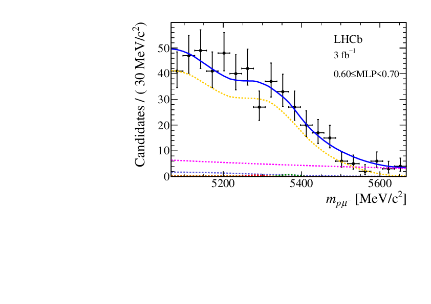
Mass distribution of signal candidates (black dots) for Run 1 samples in regions of MLP. The results of the fit described in the text are also shown.
Mass distribution of \BdToKpi candidates in data for (left) Run 1 and (right) Run 2. The results of the invariant mass fits are superimposed.
Mass distribution of signal candidates (black dots) for Run 1 samples in regions of MLP. The results of the fit described in the text are also shown.
Mass distribution of \BdToKpi candidates in data for (left) Run 1 and (right) Run 2. The results of the invariant mass fits are superimposed.
Mass distribution of signal candidates (black dots) for Run 1 samples in regions of MLP. The results of the fit described in the text are also shown.
Mass distribution of \BuToJPsiK candidates in data for (left) Run 1 and (right) Run 2. The results of the invariant mass fits are superimposed.
Mass distribution of signal candidates (black dots) for Run 1 samples in regions of MLP. The results of the fit described in the text are also shown.
Mass distribution of \BuToJPsiK candidates in data for (left) Run 1 and (right) Run 2. The results of the invariant mass fits are superimposed.
Mass distribution of signal candidates (black dots) for Run 1 samples in regions of MLP. The results of the fit described in the text are also shown.
Mass distribution of signal candidates (black dots) for Run 1 samples in regions of MLP. The results of the fit described in the text are also shown. The contributions from the two signal channels, \BdTopmu(red dashed lines) and \BsTopmu(green dashed lines), are scaled by a factor of 10 for better visibility.
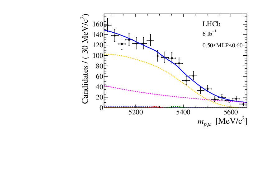
Mass distribution of signal candidates (black dots) for Run 2 samples in regions of MLP. The results of the fit described in the text are also shown.
Mass distribution of signal candidates (black dots) for Run 2 samples in regions of MLP. The results of the fit described in the text are also shown. The contributions from the two signal channels, \BdTopmu(red dashed lines) and \BsTopmu(green dashed lines), are scaled by a factor of 10 for better visibility.
Results from the CLs scan used to obtain the limit on (left) $\BR(\BdTopmu)$ and (right) $\BR(\BsTopmu)$. The background-only expectation is shown by the red line and the 1$\sigma$ and 2$\sigma$ bands are shown as light blue and blue bands respectively. The observation is shown as the solid black line. The two dashed lines intersecting with the observation indicate the limits at 90\% and 95\% CL for the upper and lower line, respectively.