Testing SO(10)-inspired leptogenesis with low energy neutrino experiments
- Di Bari, Pasquale et al
- arXiv:1012.2343
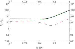
 | Case $V_L=I$. Dependence of $\eta_B^{T\sim M_2}$ (dashed line) and of $\eta_B^{\rm f}$ (solid line) on $m_1$ for the three sets of values of the parameters as in Fig.~4 of Ref. \cite{SO10}: $\theta_{13}=5^{\circ},\theta_{23}=40^{\circ}$ $\theta_{12}=33.5^{\circ}$ in all three cases. The values of the phases are different in the three panels: $\delta=\sigma=0^{\circ}, \rho=1.5^{\circ}$ (left); $\delta=5.86^{\circ}, \rho=\sigma=3^{\circ}$ (center); $\delta=\pi/3,\rho=0.02^{\circ},\sigma=\pi/2$ (right). The dotted line is the $2\sigma$ lowest value $\eta_B^{CMB}=5.9\times 10^{-10}$ (cf. (\ref{etaBobs})). |
 | Case $V_L=I$. Dependence of $\eta_B^{T\sim M_2}$ (dashed line) and of $\eta_B^{\rm f}$ (solid line) on $m_1$ for the three sets of values of the parameters as in Fig.~4 of Ref. \cite{SO10}: $\theta_{13}=5^{\circ},\theta_{23}=40^{\circ}$ $\theta_{12}=33.5^{\circ}$ in all three cases. The values of the phases are different in the three panels: $\delta=\sigma=0^{\circ}, \rho=1.5^{\circ}$ (left); $\delta=5.86^{\circ}, \rho=\sigma=3^{\circ}$ (center); $\delta=\pi/3,\rho=0.02^{\circ},\sigma=\pi/2$ (right). The dotted line is the $2\sigma$ lowest value $\eta_B^{CMB}=5.9\times 10^{-10}$ (cf. (\ref{etaBobs})). |
 | Case $V_L=I$. Dependence of $\eta_B^{T\sim M_2}$ (dashed line) and of $\eta_B^{\rm f}$ (solid line) on $m_1$ for the three sets of values of the parameters as in Fig.~4 of Ref. \cite{SO10}: $\theta_{13}=5^{\circ},\theta_{23}=40^{\circ}$ $\theta_{12}=33.5^{\circ}$ in all three cases. The values of the phases are different in the three panels: $\delta=\sigma=0^{\circ}, \rho=1.5^{\circ}$ (left); $\delta=5.86^{\circ}, \rho=\sigma=3^{\circ}$ (center); $\delta=\pi/3,\rho=0.02^{\circ},\sigma=\pi/2$ (right). The dotted line is the $2\sigma$ lowest value $\eta_B^{CMB}=5.9\times 10^{-10}$ (cf. (\ref{etaBobs})). |
 | Case $V_L=I$, NO. Scatter plot of points in the parameter space that satisfy the condition $\eta_B>5.9\times 10^{-9}$ for three values of the crucial parameter $\a_2$: $\a_2=5$ (yellow circles); $\a_2=4$ (green circles); $\a_2=3.4$ (red stars). In the top left panel the lower bound on $T_{RH}$ (cf. eq.~(\ref{TRHmin})) is also indicated for the same values of $\alpha_2$ but with different symbols: $\a_2=5$ (grey squares), $\a_2=4$ (black squares), $\a_2=3.4$ (blue star). The three mixing angles are in degrees, the three phases in radiants. The dashed line in the left central panel is the eq.~(\ref{linear}). |
 | Case $V_L=I$, NO. Scatter plot of points in the parameter space that satisfy the condition $\eta_B>5.9\times 10^{-9}$ for three values of the crucial parameter $\a_2$: $\a_2=5$ (yellow circles); $\a_2=4$ (green circles); $\a_2=3.4$ (red stars). In the top left panel the lower bound on $T_{RH}$ (cf. eq.~(\ref{TRHmin})) is also indicated for the same values of $\alpha_2$ but with different symbols: $\a_2=5$ (grey squares), $\a_2=4$ (black squares), $\a_2=3.4$ (blue star). The three mixing angles are in degrees, the three phases in radiants. The dashed line in the left central panel is the eq.~(\ref{linear}). |
 | Case $V_L=I$, NO. Scatter plot of points in the parameter space that satisfy the condition $\eta_B>5.9\times 10^{-9}$ for three values of the crucial parameter $\a_2$: $\a_2=5$ (yellow circles); $\a_2=4$ (green circles); $\a_2=3.4$ (red stars). In the top left panel the lower bound on $T_{RH}$ (cf. eq.~(\ref{TRHmin})) is also indicated for the same values of $\alpha_2$ but with different symbols: $\a_2=5$ (grey squares), $\a_2=4$ (black squares), $\a_2=3.4$ (blue star). The three mixing angles are in degrees, the three phases in radiants. The dashed line in the left central panel is the eq.~(\ref{linear}). |
 | Case $V_L=I$, NO. Scatter plot of points in the parameter space that satisfy the condition $\eta_B>5.9\times 10^{-9}$ for three values of the crucial parameter $\a_2$: $\a_2=5$ (yellow circles); $\a_2=4$ (green circles); $\a_2=3.4$ (red stars). In the top left panel the lower bound on $T_{RH}$ (cf. eq.~(\ref{TRHmin})) is also indicated for the same values of $\alpha_2$ but with different symbols: $\a_2=5$ (grey squares), $\a_2=4$ (black squares), $\a_2=3.4$ (blue star). The three mixing angles are in degrees, the three phases in radiants. The dashed line in the left central panel is the eq.~(\ref{linear}). |
 | Case $V_L=I$, NO. Scatter plot of points in the parameter space that satisfy the condition $\eta_B>5.9\times 10^{-9}$ for three values of the crucial parameter $\a_2$: $\a_2=5$ (yellow circles); $\a_2=4$ (green circles); $\a_2=3.4$ (red stars). In the top left panel the lower bound on $T_{RH}$ (cf. eq.~(\ref{TRHmin})) is also indicated for the same values of $\alpha_2$ but with different symbols: $\a_2=5$ (grey squares), $\a_2=4$ (black squares), $\a_2=3.4$ (blue star). The three mixing angles are in degrees, the three phases in radiants. The dashed line in the left central panel is the eq.~(\ref{linear}). |
 | Case $V_L=I$, NO. Scatter plot of points in the parameter space that satisfy the condition $\eta_B>5.9\times 10^{-9}$ for three values of the crucial parameter $\a_2$: $\a_2=5$ (yellow circles); $\a_2=4$ (green circles); $\a_2=3.4$ (red stars). In the top left panel the lower bound on $T_{RH}$ (cf. eq.~(\ref{TRHmin})) is also indicated for the same values of $\alpha_2$ but with different symbols: $\a_2=5$ (grey squares), $\a_2=4$ (black squares), $\a_2=3.4$ (blue star). The three mixing angles are in degrees, the three phases in radiants. The dashed line in the left central panel is the eq.~(\ref{linear}). |
 | Case $V_L=I$, NO. Scatter plot of points in the parameter space that satisfy the condition $\eta_B>5.9\times 10^{-9}$ for three values of the crucial parameter $\a_2$: $\a_2=5$ (yellow circles); $\a_2=4$ (green circles); $\a_2=3.4$ (red stars). In the top left panel the lower bound on $T_{RH}$ (cf. eq.~(\ref{TRHmin})) is also indicated for the same values of $\alpha_2$ but with different symbols: $\a_2=5$ (grey squares), $\a_2=4$ (black squares), $\a_2=3.4$ (blue star). The three mixing angles are in degrees, the three phases in radiants. The dashed line in the left central panel is the eq.~(\ref{linear}). |
 | Case $V_L=I$, NO. Scatter plot of points in the parameter space that satisfy the condition $\eta_B>5.9\times 10^{-9}$ for three values of the crucial parameter $\a_2$: $\a_2=5$ (yellow circles); $\a_2=4$ (green circles); $\a_2=3.4$ (red stars). In the top left panel the lower bound on $T_{RH}$ (cf. eq.~(\ref{TRHmin})) is also indicated for the same values of $\alpha_2$ but with different symbols: $\a_2=5$ (grey squares), $\a_2=4$ (black squares), $\a_2=3.4$ (blue star). The three mixing angles are in degrees, the three phases in radiants. The dashed line in the left central panel is the eq.~(\ref{linear}). |
 | Case $V_L=I$, NO. Scatter plot of points in the parameter space that satisfy the condition $\eta_B>5.9\times 10^{-9}$ for three values of the crucial parameter $\a_2$: $\a_2=5$ (yellow circles); $\a_2=4$ (green circles); $\a_2=3.4$ (red stars). In the top left panel the lower bound on $T_{RH}$ (cf. eq.~(\ref{TRHmin})) is also indicated for the same values of $\alpha_2$ but with different symbols: $\a_2=5$ (grey squares), $\a_2=4$ (black squares), $\a_2=3.4$ (blue star). The three mixing angles are in degrees, the three phases in radiants. The dashed line in the left central panel is the eq.~(\ref{linear}). |
 | Case $V_L=1$, NO, $\a_2=4$. Constraints on the mixing angles obtained without imposing the current experimental information from neutrino oscillation experiments (blue points) compared to those previously obtained (green points). |
 | Case $V_L=1$, NO, $\a_2=4$. Constraints on the mixing angles obtained without imposing the current experimental information from neutrino oscillation experiments (blue points) compared to those previously obtained (green points). |
 | Case $V_L=1$, NO, $\a_2=4$. Constraints on the mixing angles obtained without imposing the current experimental information from neutrino oscillation experiments (blue points) compared to those previously obtained (green points). |
 | Case $V_L=I$, IO. Scatter plot of points in the parameter space that satisfy the condition $\eta_B>5.9\times 10^{-9}$ for $\a_2=5$ (yellow circles) and $\a_2=4.65$ (red star). In the top left panel the lower bound on $T_{RH}$ (cf. eq.~(\ref{TRHmin})) is also indicated for the same values of $\alpha_2$ but with different symbols: $\a_2=5$ (grey squares), $\a_2=4.65$ (blue star). The three mixing angles are in degrees, the three phases in radiant. |
 | Case $V_L=I$, IO. Scatter plot of points in the parameter space that satisfy the condition $\eta_B>5.9\times 10^{-9}$ for $\a_2=5$ (yellow circles) and $\a_2=4.65$ (red star). In the top left panel the lower bound on $T_{RH}$ (cf. eq.~(\ref{TRHmin})) is also indicated for the same values of $\alpha_2$ but with different symbols: $\a_2=5$ (grey squares), $\a_2=4.65$ (blue star). The three mixing angles are in degrees, the three phases in radiant. |
 | Case $V_L=I$, IO. Scatter plot of points in the parameter space that satisfy the condition $\eta_B>5.9\times 10^{-9}$ for $\a_2=5$ (yellow circles) and $\a_2=4.65$ (red star). In the top left panel the lower bound on $T_{RH}$ (cf. eq.~(\ref{TRHmin})) is also indicated for the same values of $\alpha_2$ but with different symbols: $\a_2=5$ (grey squares), $\a_2=4.65$ (blue star). The three mixing angles are in degrees, the three phases in radiant. |
 | Case $V_L=I$, IO. Scatter plot of points in the parameter space that satisfy the condition $\eta_B>5.9\times 10^{-9}$ for $\a_2=5$ (yellow circles) and $\a_2=4.65$ (red star). In the top left panel the lower bound on $T_{RH}$ (cf. eq.~(\ref{TRHmin})) is also indicated for the same values of $\alpha_2$ but with different symbols: $\a_2=5$ (grey squares), $\a_2=4.65$ (blue star). The three mixing angles are in degrees, the three phases in radiant. |
 | Case $V_L=I$, IO. Scatter plot of points in the parameter space that satisfy the condition $\eta_B>5.9\times 10^{-9}$ for $\a_2=5$ (yellow circles) and $\a_2=4.65$ (red star). In the top left panel the lower bound on $T_{RH}$ (cf. eq.~(\ref{TRHmin})) is also indicated for the same values of $\alpha_2$ but with different symbols: $\a_2=5$ (grey squares), $\a_2=4.65$ (blue star). The three mixing angles are in degrees, the three phases in radiant. |
 | Case $V_L=I$, IO. Scatter plot of points in the parameter space that satisfy the condition $\eta_B>5.9\times 10^{-9}$ for $\a_2=5$ (yellow circles) and $\a_2=4.65$ (red star). In the top left panel the lower bound on $T_{RH}$ (cf. eq.~(\ref{TRHmin})) is also indicated for the same values of $\alpha_2$ but with different symbols: $\a_2=5$ (grey squares), $\a_2=4.65$ (blue star). The three mixing angles are in degrees, the three phases in radiant. |
 | Case $V_L=I$, IO. Scatter plot of points in the parameter space that satisfy the condition $\eta_B>5.9\times 10^{-9}$ for $\a_2=5$ (yellow circles) and $\a_2=4.65$ (red star). In the top left panel the lower bound on $T_{RH}$ (cf. eq.~(\ref{TRHmin})) is also indicated for the same values of $\alpha_2$ but with different symbols: $\a_2=5$ (grey squares), $\a_2=4.65$ (blue star). The three mixing angles are in degrees, the three phases in radiant. |
 | Case $V_L=I$, IO. Scatter plot of points in the parameter space that satisfy the condition $\eta_B>5.9\times 10^{-9}$ for $\a_2=5$ (yellow circles) and $\a_2=4.65$ (red star). In the top left panel the lower bound on $T_{RH}$ (cf. eq.~(\ref{TRHmin})) is also indicated for the same values of $\alpha_2$ but with different symbols: $\a_2=5$ (grey squares), $\a_2=4.65$ (blue star). The three mixing angles are in degrees, the three phases in radiant. |
 | Case $V_L=I$, IO. Scatter plot of points in the parameter space that satisfy the condition $\eta_B>5.9\times 10^{-9}$ for $\a_2=5$ (yellow circles) and $\a_2=4.65$ (red star). In the top left panel the lower bound on $T_{RH}$ (cf. eq.~(\ref{TRHmin})) is also indicated for the same values of $\alpha_2$ but with different symbols: $\a_2=5$ (grey squares), $\a_2=4.65$ (blue star). The three mixing angles are in degrees, the three phases in radiant. |
 | Case $V_L=I$, IO. Plot of all relevant quantities versus $m_1$ for the set of values ($\theta_{13}=0.32^{\circ}$,$\theta_{23}=52.03^{\circ}$,$\theta_{12}=32.16^{\circ}$, $\rho=3.16$,$\sigma=3.48$,$\delta=2.47$) corresponding to the red star in the previous figure ($\a_2=4.65$). |
 | Case $V_L=I$, IO. Plot of all relevant quantities versus $m_1$ for the set of values ($\theta_{13}=0.32^{\circ}$,$\theta_{23}=52.03^{\circ}$,$\theta_{12}=32.16^{\circ}$, $\rho=3.16$,$\sigma=3.48$,$\delta=2.47$) corresponding to the red star in the previous figure ($\a_2=4.65$). |
 | Case $V_L=I$, IO. Plot of all relevant quantities versus $m_1$ for the set of values ($\theta_{13}=0.32^{\circ}$,$\theta_{23}=52.03^{\circ}$,$\theta_{12}=32.16^{\circ}$, $\rho=3.16$,$\sigma=3.48$,$\delta=2.47$) corresponding to the red star in the previous figure ($\a_2=4.65$). |
 | Case $V_L=I$, IO. Plot of all relevant quantities versus $m_1$ for the set of values ($\theta_{13}=0.32^{\circ}$,$\theta_{23}=52.03^{\circ}$,$\theta_{12}=32.16^{\circ}$, $\rho=3.16$,$\sigma=3.48$,$\delta=2.47$) corresponding to the red star in the previous figure ($\a_2=4.65$). |
 | Case $V_L=I$, IO. Plot of all relevant quantities versus $m_1$ for the set of values ($\theta_{13}=0.32^{\circ}$,$\theta_{23}=52.03^{\circ}$,$\theta_{12}=32.16^{\circ}$, $\rho=3.16$,$\sigma=3.48$,$\delta=2.47$) corresponding to the red star in the previous figure ($\a_2=4.65$). |
 | Case $V_L=V_{CKM}$, NO. Scatter plot of points in the parameter space that satisfy the condition $\eta_B>5.9\times 10^{-9}$ for $\a_2=5$ (yellow circles), $\a_2=4$ (green squares) and $\a_2=1$ (red stars). |
 | Case $V_L=V_{CKM}$, NO. Scatter plot of points in the parameter space that satisfy the condition $\eta_B>5.9\times 10^{-9}$ for $\a_2=5$ (yellow circles), $\a_2=4$ (green squares) and $\a_2=1$ (red stars). |
 | Case $V_L=V_{CKM}$, NO. Scatter plot of points in the parameter space that satisfy the condition $\eta_B>5.9\times 10^{-9}$ for $\a_2=5$ (yellow circles), $\a_2=4$ (green squares) and $\a_2=1$ (red stars). |
 | Case $V_L=V_{CKM}$, NO. Scatter plot of points in the parameter space that satisfy the condition $\eta_B>5.9\times 10^{-9}$ for $\a_2=5$ (yellow circles), $\a_2=4$ (green squares) and $\a_2=1$ (red stars). |
 | Case $V_L=V_{CKM}$, NO. Scatter plot of points in the parameter space that satisfy the condition $\eta_B>5.9\times 10^{-9}$ for $\a_2=5$ (yellow circles), $\a_2=4$ (green squares) and $\a_2=1$ (red stars). |
 | Case $V_L=V_{CKM}$, NO. Scatter plot of points in the parameter space that satisfy the condition $\eta_B>5.9\times 10^{-9}$ for $\a_2=5$ (yellow circles), $\a_2=4$ (green squares) and $\a_2=1$ (red stars). |
 | Case $V_L=V_{CKM}$, NO. Scatter plot of points in the parameter space that satisfy the condition $\eta_B>5.9\times 10^{-9}$ for $\a_2=5$ (yellow circles), $\a_2=4$ (green squares) and $\a_2=1$ (red stars). |
 | Case $V_L=V_{CKM}$, NO. Scatter plot of points in the parameter space that satisfy the condition $\eta_B>5.9\times 10^{-9}$ for $\a_2=5$ (yellow circles), $\a_2=4$ (green squares) and $\a_2=1$ (red stars). |
 | Case $V_L=V_{CKM}$, NO. Scatter plot of points in the parameter space that satisfy the condition $\eta_B>5.9\times 10^{-9}$ for $\a_2=5$ (yellow circles), $\a_2=4$ (green squares) and $\a_2=1$ (red stars). |
 | Case $V_L=V_{CKM}$, NO. Plots of the relevant quantities for three choices of the involved parameters. The long-dashed red lines correspond to $\a=\t$, the dashed blue lines to $\a=\m$ and the short-dashed dark yellow lines to $\a=e$. Left panels: $\a_2=4$, $\theta_{13}=1.7^{\circ}$, $\theta_{12}=33.6^{\circ}$, $\theta_{23}=41.8^{\circ}$, $\d=2.84$, $\rho=$1.53 $\sigma=3.24$, $\rho_L=0.12$, $\sigma_L=2.56$; central panels: $\a_2=5$, $\theta_{13}=3.3^{\circ}$, $\theta_{12}=35.6^{\circ}$, $\theta_{23}=40.4^{\circ}$, $\d=-1.06$, $\rho=2.87$, $\sigma=6.0$, $\rho_L=3.13$, $\sigma_L=3.25$; right panels: $\a_2=4$, $\theta_{13}=4.7^{\circ}$, $\theta_{12}=35.9^{\circ}$, $\theta_{23}=40.3^{\circ}$, $\d=-1.89$, $\rho=0.065$, $\sigma=4.85$, $\rho_L=5.89$, $\sigma_L=3.69$. |
 | Case $V_L=V_{CKM}$, NO. Plots of the relevant quantities for three choices of the involved parameters. The long-dashed red lines correspond to $\a=\t$, the dashed blue lines to $\a=\m$ and the short-dashed dark yellow lines to $\a=e$. Left panels: $\a_2=4$, $\theta_{13}=1.7^{\circ}$, $\theta_{12}=33.6^{\circ}$, $\theta_{23}=41.8^{\circ}$, $\d=2.84$, $\rho=$1.53 $\sigma=3.24$, $\rho_L=0.12$, $\sigma_L=2.56$; central panels: $\a_2=5$, $\theta_{13}=3.3^{\circ}$, $\theta_{12}=35.6^{\circ}$, $\theta_{23}=40.4^{\circ}$, $\d=-1.06$, $\rho=2.87$, $\sigma=6.0$, $\rho_L=3.13$, $\sigma_L=3.25$; right panels: $\a_2=4$, $\theta_{13}=4.7^{\circ}$, $\theta_{12}=35.9^{\circ}$, $\theta_{23}=40.3^{\circ}$, $\d=-1.89$, $\rho=0.065$, $\sigma=4.85$, $\rho_L=5.89$, $\sigma_L=3.69$. |
 | Case $V_L=V_{CKM}$, NO. Plots of the relevant quantities for three choices of the involved parameters. The long-dashed red lines correspond to $\a=\t$, the dashed blue lines to $\a=\m$ and the short-dashed dark yellow lines to $\a=e$. Left panels: $\a_2=4$, $\theta_{13}=1.7^{\circ}$, $\theta_{12}=33.6^{\circ}$, $\theta_{23}=41.8^{\circ}$, $\d=2.84$, $\rho=$1.53 $\sigma=3.24$, $\rho_L=0.12$, $\sigma_L=2.56$; central panels: $\a_2=5$, $\theta_{13}=3.3^{\circ}$, $\theta_{12}=35.6^{\circ}$, $\theta_{23}=40.4^{\circ}$, $\d=-1.06$, $\rho=2.87$, $\sigma=6.0$, $\rho_L=3.13$, $\sigma_L=3.25$; right panels: $\a_2=4$, $\theta_{13}=4.7^{\circ}$, $\theta_{12}=35.9^{\circ}$, $\theta_{23}=40.3^{\circ}$, $\d=-1.89$, $\rho=0.065$, $\sigma=4.85$, $\rho_L=5.89$, $\sigma_L=3.69$. |
 | Case $V_L=V_{CKM}$, NO. Plots of the relevant quantities for three choices of the involved parameters. The long-dashed red lines correspond to $\a=\t$, the dashed blue lines to $\a=\m$ and the short-dashed dark yellow lines to $\a=e$. Left panels: $\a_2=4$, $\theta_{13}=1.7^{\circ}$, $\theta_{12}=33.6^{\circ}$, $\theta_{23}=41.8^{\circ}$, $\d=2.84$, $\rho=$1.53 $\sigma=3.24$, $\rho_L=0.12$, $\sigma_L=2.56$; central panels: $\a_2=5$, $\theta_{13}=3.3^{\circ}$, $\theta_{12}=35.6^{\circ}$, $\theta_{23}=40.4^{\circ}$, $\d=-1.06$, $\rho=2.87$, $\sigma=6.0$, $\rho_L=3.13$, $\sigma_L=3.25$; right panels: $\a_2=4$, $\theta_{13}=4.7^{\circ}$, $\theta_{12}=35.9^{\circ}$, $\theta_{23}=40.3^{\circ}$, $\d=-1.89$, $\rho=0.065$, $\sigma=4.85$, $\rho_L=5.89$, $\sigma_L=3.69$. |
 | Case $V_L=V_{CKM}$, NO. Plots of the relevant quantities for three choices of the involved parameters. The long-dashed red lines correspond to $\a=\t$, the dashed blue lines to $\a=\m$ and the short-dashed dark yellow lines to $\a=e$. Left panels: $\a_2=4$, $\theta_{13}=1.7^{\circ}$, $\theta_{12}=33.6^{\circ}$, $\theta_{23}=41.8^{\circ}$, $\d=2.84$, $\rho=$1.53 $\sigma=3.24$, $\rho_L=0.12$, $\sigma_L=2.56$; central panels: $\a_2=5$, $\theta_{13}=3.3^{\circ}$, $\theta_{12}=35.6^{\circ}$, $\theta_{23}=40.4^{\circ}$, $\d=-1.06$, $\rho=2.87$, $\sigma=6.0$, $\rho_L=3.13$, $\sigma_L=3.25$; right panels: $\a_2=4$, $\theta_{13}=4.7^{\circ}$, $\theta_{12}=35.9^{\circ}$, $\theta_{23}=40.3^{\circ}$, $\d=-1.89$, $\rho=0.065$, $\sigma=4.85$, $\rho_L=5.89$, $\sigma_L=3.69$. |
 | Case $V_L=V_{CKM}$, NO. Plots of the relevant quantities for three choices of the involved parameters. The long-dashed red lines correspond to $\a=\t$, the dashed blue lines to $\a=\m$ and the short-dashed dark yellow lines to $\a=e$. Left panels: $\a_2=4$, $\theta_{13}=1.7^{\circ}$, $\theta_{12}=33.6^{\circ}$, $\theta_{23}=41.8^{\circ}$, $\d=2.84$, $\rho=$1.53 $\sigma=3.24$, $\rho_L=0.12$, $\sigma_L=2.56$; central panels: $\a_2=5$, $\theta_{13}=3.3^{\circ}$, $\theta_{12}=35.6^{\circ}$, $\theta_{23}=40.4^{\circ}$, $\d=-1.06$, $\rho=2.87$, $\sigma=6.0$, $\rho_L=3.13$, $\sigma_L=3.25$; right panels: $\a_2=4$, $\theta_{13}=4.7^{\circ}$, $\theta_{12}=35.9^{\circ}$, $\theta_{23}=40.3^{\circ}$, $\d=-1.89$, $\rho=0.065$, $\sigma=4.85$, $\rho_L=5.89$, $\sigma_L=3.69$. |
 | Case $V_L=V_{CKM}$, NO. Plots of the relevant quantities for three choices of the involved parameters. The long-dashed red lines correspond to $\a=\t$, the dashed blue lines to $\a=\m$ and the short-dashed dark yellow lines to $\a=e$. Left panels: $\a_2=4$, $\theta_{13}=1.7^{\circ}$, $\theta_{12}=33.6^{\circ}$, $\theta_{23}=41.8^{\circ}$, $\d=2.84$, $\rho=$1.53 $\sigma=3.24$, $\rho_L=0.12$, $\sigma_L=2.56$; central panels: $\a_2=5$, $\theta_{13}=3.3^{\circ}$, $\theta_{12}=35.6^{\circ}$, $\theta_{23}=40.4^{\circ}$, $\d=-1.06$, $\rho=2.87$, $\sigma=6.0$, $\rho_L=3.13$, $\sigma_L=3.25$; right panels: $\a_2=4$, $\theta_{13}=4.7^{\circ}$, $\theta_{12}=35.9^{\circ}$, $\theta_{23}=40.3^{\circ}$, $\d=-1.89$, $\rho=0.065$, $\sigma=4.85$, $\rho_L=5.89$, $\sigma_L=3.69$. |
 | Case $V_L=V_{CKM}$, NO. Plots of the relevant quantities for three choices of the involved parameters. The long-dashed red lines correspond to $\a=\t$, the dashed blue lines to $\a=\m$ and the short-dashed dark yellow lines to $\a=e$. Left panels: $\a_2=4$, $\theta_{13}=1.7^{\circ}$, $\theta_{12}=33.6^{\circ}$, $\theta_{23}=41.8^{\circ}$, $\d=2.84$, $\rho=$1.53 $\sigma=3.24$, $\rho_L=0.12$, $\sigma_L=2.56$; central panels: $\a_2=5$, $\theta_{13}=3.3^{\circ}$, $\theta_{12}=35.6^{\circ}$, $\theta_{23}=40.4^{\circ}$, $\d=-1.06$, $\rho=2.87$, $\sigma=6.0$, $\rho_L=3.13$, $\sigma_L=3.25$; right panels: $\a_2=4$, $\theta_{13}=4.7^{\circ}$, $\theta_{12}=35.9^{\circ}$, $\theta_{23}=40.3^{\circ}$, $\d=-1.89$, $\rho=0.065$, $\sigma=4.85$, $\rho_L=5.89$, $\sigma_L=3.69$. |
 | Case $V_L=V_{CKM}$, NO. Plots of the relevant quantities for three choices of the involved parameters. The long-dashed red lines correspond to $\a=\t$, the dashed blue lines to $\a=\m$ and the short-dashed dark yellow lines to $\a=e$. Left panels: $\a_2=4$, $\theta_{13}=1.7^{\circ}$, $\theta_{12}=33.6^{\circ}$, $\theta_{23}=41.8^{\circ}$, $\d=2.84$, $\rho=$1.53 $\sigma=3.24$, $\rho_L=0.12$, $\sigma_L=2.56$; central panels: $\a_2=5$, $\theta_{13}=3.3^{\circ}$, $\theta_{12}=35.6^{\circ}$, $\theta_{23}=40.4^{\circ}$, $\d=-1.06$, $\rho=2.87$, $\sigma=6.0$, $\rho_L=3.13$, $\sigma_L=3.25$; right panels: $\a_2=4$, $\theta_{13}=4.7^{\circ}$, $\theta_{12}=35.9^{\circ}$, $\theta_{23}=40.3^{\circ}$, $\d=-1.89$, $\rho=0.065$, $\sigma=4.85$, $\rho_L=5.89$, $\sigma_L=3.69$. |
 | Case $V_L=V_{CKM}$, NO. Plots of the relevant quantities for three choices of the involved parameters. The long-dashed red lines correspond to $\a=\t$, the dashed blue lines to $\a=\m$ and the short-dashed dark yellow lines to $\a=e$. Left panels: $\a_2=4$, $\theta_{13}=1.7^{\circ}$, $\theta_{12}=33.6^{\circ}$, $\theta_{23}=41.8^{\circ}$, $\d=2.84$, $\rho=$1.53 $\sigma=3.24$, $\rho_L=0.12$, $\sigma_L=2.56$; central panels: $\a_2=5$, $\theta_{13}=3.3^{\circ}$, $\theta_{12}=35.6^{\circ}$, $\theta_{23}=40.4^{\circ}$, $\d=-1.06$, $\rho=2.87$, $\sigma=6.0$, $\rho_L=3.13$, $\sigma_L=3.25$; right panels: $\a_2=4$, $\theta_{13}=4.7^{\circ}$, $\theta_{12}=35.9^{\circ}$, $\theta_{23}=40.3^{\circ}$, $\d=-1.89$, $\rho=0.065$, $\sigma=4.85$, $\rho_L=5.89$, $\sigma_L=3.69$. |
 | Case $V_L=V_{CKM}$, NO. Plots of the relevant quantities for three choices of the involved parameters. The long-dashed red lines correspond to $\a=\t$, the dashed blue lines to $\a=\m$ and the short-dashed dark yellow lines to $\a=e$. Left panels: $\a_2=4$, $\theta_{13}=1.7^{\circ}$, $\theta_{12}=33.6^{\circ}$, $\theta_{23}=41.8^{\circ}$, $\d=2.84$, $\rho=$1.53 $\sigma=3.24$, $\rho_L=0.12$, $\sigma_L=2.56$; central panels: $\a_2=5$, $\theta_{13}=3.3^{\circ}$, $\theta_{12}=35.6^{\circ}$, $\theta_{23}=40.4^{\circ}$, $\d=-1.06$, $\rho=2.87$, $\sigma=6.0$, $\rho_L=3.13$, $\sigma_L=3.25$; right panels: $\a_2=4$, $\theta_{13}=4.7^{\circ}$, $\theta_{12}=35.9^{\circ}$, $\theta_{23}=40.3^{\circ}$, $\d=-1.89$, $\rho=0.065$, $\sigma=4.85$, $\rho_L=5.89$, $\sigma_L=3.69$. |
 | Case $V_L=V_{CKM}$, NO. Plots of the relevant quantities for three choices of the involved parameters. The long-dashed red lines correspond to $\a=\t$, the dashed blue lines to $\a=\m$ and the short-dashed dark yellow lines to $\a=e$. Left panels: $\a_2=4$, $\theta_{13}=1.7^{\circ}$, $\theta_{12}=33.6^{\circ}$, $\theta_{23}=41.8^{\circ}$, $\d=2.84$, $\rho=$1.53 $\sigma=3.24$, $\rho_L=0.12$, $\sigma_L=2.56$; central panels: $\a_2=5$, $\theta_{13}=3.3^{\circ}$, $\theta_{12}=35.6^{\circ}$, $\theta_{23}=40.4^{\circ}$, $\d=-1.06$, $\rho=2.87$, $\sigma=6.0$, $\rho_L=3.13$, $\sigma_L=3.25$; right panels: $\a_2=4$, $\theta_{13}=4.7^{\circ}$, $\theta_{12}=35.9^{\circ}$, $\theta_{23}=40.3^{\circ}$, $\d=-1.89$, $\rho=0.065$, $\sigma=4.85$, $\rho_L=5.89$, $\sigma_L=3.69$. |
 | Case $V_L=V_{CKM}$, NO. Plots of the relevant quantities for three choices of the involved parameters. The long-dashed red lines correspond to $\a=\t$, the dashed blue lines to $\a=\m$ and the short-dashed dark yellow lines to $\a=e$. Left panels: $\a_2=4$, $\theta_{13}=1.7^{\circ}$, $\theta_{12}=33.6^{\circ}$, $\theta_{23}=41.8^{\circ}$, $\d=2.84$, $\rho=$1.53 $\sigma=3.24$, $\rho_L=0.12$, $\sigma_L=2.56$; central panels: $\a_2=5$, $\theta_{13}=3.3^{\circ}$, $\theta_{12}=35.6^{\circ}$, $\theta_{23}=40.4^{\circ}$, $\d=-1.06$, $\rho=2.87$, $\sigma=6.0$, $\rho_L=3.13$, $\sigma_L=3.25$; right panels: $\a_2=4$, $\theta_{13}=4.7^{\circ}$, $\theta_{12}=35.9^{\circ}$, $\theta_{23}=40.3^{\circ}$, $\d=-1.89$, $\rho=0.065$, $\sigma=4.85$, $\rho_L=5.89$, $\sigma_L=3.69$. |
 | Case $V_L=V_{CKM}$, NO. Plots of the relevant quantities for three choices of the involved parameters. The long-dashed red lines correspond to $\a=\t$, the dashed blue lines to $\a=\m$ and the short-dashed dark yellow lines to $\a=e$. Left panels: $\a_2=4$, $\theta_{13}=1.7^{\circ}$, $\theta_{12}=33.6^{\circ}$, $\theta_{23}=41.8^{\circ}$, $\d=2.84$, $\rho=$1.53 $\sigma=3.24$, $\rho_L=0.12$, $\sigma_L=2.56$; central panels: $\a_2=5$, $\theta_{13}=3.3^{\circ}$, $\theta_{12}=35.6^{\circ}$, $\theta_{23}=40.4^{\circ}$, $\d=-1.06$, $\rho=2.87$, $\sigma=6.0$, $\rho_L=3.13$, $\sigma_L=3.25$; right panels: $\a_2=4$, $\theta_{13}=4.7^{\circ}$, $\theta_{12}=35.9^{\circ}$, $\theta_{23}=40.3^{\circ}$, $\d=-1.89$, $\rho=0.065$, $\sigma=4.85$, $\rho_L=5.89$, $\sigma_L=3.69$. |
 | Case $V_L=V_{CKM}$, NO. Plots of the relevant quantities for three choices of the involved parameters. The long-dashed red lines correspond to $\a=\t$, the dashed blue lines to $\a=\m$ and the short-dashed dark yellow lines to $\a=e$. Left panels: $\a_2=4$, $\theta_{13}=1.7^{\circ}$, $\theta_{12}=33.6^{\circ}$, $\theta_{23}=41.8^{\circ}$, $\d=2.84$, $\rho=$1.53 $\sigma=3.24$, $\rho_L=0.12$, $\sigma_L=2.56$; central panels: $\a_2=5$, $\theta_{13}=3.3^{\circ}$, $\theta_{12}=35.6^{\circ}$, $\theta_{23}=40.4^{\circ}$, $\d=-1.06$, $\rho=2.87$, $\sigma=6.0$, $\rho_L=3.13$, $\sigma_L=3.25$; right panels: $\a_2=4$, $\theta_{13}=4.7^{\circ}$, $\theta_{12}=35.9^{\circ}$, $\theta_{23}=40.3^{\circ}$, $\d=-1.89$, $\rho=0.065$, $\sigma=4.85$, $\rho_L=5.89$, $\sigma_L=3.69$. |
 | Case $V_L=V_{CKM}$, NO. Constraints on the mixing angles without making use of the current experimental information from neutrino oscillation experiments. |
 | Case $V_L=V_{CKM}$, NO. Constraints on the mixing angles without making use of the current experimental information from neutrino oscillation experiments. |
 | Case $V_L=V_{CKM}$, NO. Constraints on the mixing angles without making use of the current experimental information from neutrino oscillation experiments. |
 | Case $V_L=V_{CKM}$, IO. Scatter plot of points in the parameter space that satisfy the condition $\eta_B>5.9\times 10^{-9}$ for $\a_2=5$ (yellow circles), $\a_2=4$ (green squares) and $\a_2= 2$ (red star). |
 | Case $V_L=V_{CKM}$, IO. Scatter plot of points in the parameter space that satisfy the condition $\eta_B>5.9\times 10^{-9}$ for $\a_2=5$ (yellow circles), $\a_2=4$ (green squares) and $\a_2= 2$ (red star). |
 | Case $V_L=V_{CKM}$, IO. Scatter plot of points in the parameter space that satisfy the condition $\eta_B>5.9\times 10^{-9}$ for $\a_2=5$ (yellow circles), $\a_2=4$ (green squares) and $\a_2= 2$ (red star). |
 | Case $V_L=V_{CKM}$, IO. Scatter plot of points in the parameter space that satisfy the condition $\eta_B>5.9\times 10^{-9}$ for $\a_2=5$ (yellow circles), $\a_2=4$ (green squares) and $\a_2= 2$ (red star). |
 | Case $V_L=V_{CKM}$, IO. Scatter plot of points in the parameter space that satisfy the condition $\eta_B>5.9\times 10^{-9}$ for $\a_2=5$ (yellow circles), $\a_2=4$ (green squares) and $\a_2= 2$ (red star). |
 | Case $V_L=V_{CKM}$, IO. Scatter plot of points in the parameter space that satisfy the condition $\eta_B>5.9\times 10^{-9}$ for $\a_2=5$ (yellow circles), $\a_2=4$ (green squares) and $\a_2= 2$ (red star). |
 | Case $V_L=V_{CKM}$, IO. Scatter plot of points in the parameter space that satisfy the condition $\eta_B>5.9\times 10^{-9}$ for $\a_2=5$ (yellow circles), $\a_2=4$ (green squares) and $\a_2= 2$ (red star). |
 | Case $V_L=V_{CKM}$, IO. Scatter plot of points in the parameter space that satisfy the condition $\eta_B>5.9\times 10^{-9}$ for $\a_2=5$ (yellow circles), $\a_2=4$ (green squares) and $\a_2= 2$ (red star). |
 | Case $V_L=V_{CKM}$, IO. Scatter plot of points in the parameter space that satisfy the condition $\eta_B>5.9\times 10^{-9}$ for $\a_2=5$ (yellow circles), $\a_2=4$ (green squares) and $\a_2= 2$ (red star). |
 | Global scan, NO. Scatter plot of points in the parameter space that satisfy successful leptogenesis ($\eta_B>5.9\times 10^{-9}$), for $\a_2=5$ (yellow circles), $\a_2=4$ (green squares) and $\a_2=1$ (red stars). |
 | Global scan, NO. Scatter plot of points in the parameter space that satisfy successful leptogenesis ($\eta_B>5.9\times 10^{-9}$), for $\a_2=5$ (yellow circles), $\a_2=4$ (green squares) and $\a_2=1$ (red stars). |
 | Global scan, NO. Scatter plot of points in the parameter space that satisfy successful leptogenesis ($\eta_B>5.9\times 10^{-9}$), for $\a_2=5$ (yellow circles), $\a_2=4$ (green squares) and $\a_2=1$ (red stars). |
 | Global scan, NO. Scatter plot of points in the parameter space that satisfy successful leptogenesis ($\eta_B>5.9\times 10^{-9}$), for $\a_2=5$ (yellow circles), $\a_2=4$ (green squares) and $\a_2=1$ (red stars). |
 | Global scan, NO. Scatter plot of points in the parameter space that satisfy successful leptogenesis ($\eta_B>5.9\times 10^{-9}$), for $\a_2=5$ (yellow circles), $\a_2=4$ (green squares) and $\a_2=1$ (red stars). |
 | Global scan, NO. Scatter plot of points in the parameter space that satisfy successful leptogenesis ($\eta_B>5.9\times 10^{-9}$), for $\a_2=5$ (yellow circles), $\a_2=4$ (green squares) and $\a_2=1$ (red stars). |
 | Global scan, NO. Scatter plot of points in the parameter space that satisfy successful leptogenesis ($\eta_B>5.9\times 10^{-9}$), for $\a_2=5$ (yellow circles), $\a_2=4$ (green squares) and $\a_2=1$ (red stars). |
 | Global scan, NO. Scatter plot of points in the parameter space that satisfy successful leptogenesis ($\eta_B>5.9\times 10^{-9}$), for $\a_2=5$ (yellow circles), $\a_2=4$ (green squares) and $\a_2=1$ (red stars). |
 | Global scan, NO. Scatter plot of points in the parameter space that satisfy successful leptogenesis ($\eta_B>5.9\times 10^{-9}$), for $\a_2=5$ (yellow circles), $\a_2=4$ (green squares) and $\a_2=1$ (red stars). |
 | Global scan, NO. Scatter plot of points in the parameter space that satisfy successful leptogenesis ($\eta_B>5.9\times 10^{-9}$), for $\a_2=5$ (yellow circles), $\a_2=4$ (green squares) and $\a_2=1$ (red stars). |
 | Global scan, NO, $m_1<0.01 \,{\rm eV}$. Scatter plot of points in the parameter space that satisfy successful leptogenesis ($\eta_B>5.9\times 10^{-9}$), for $\a_2=5$ (yellow circles), $\a_2=4$ (green squares) and $\a_2=3.7$ (red stars). The region between the two dashed lines in the left central panel describes graphically the condition eq.~(\ref{linear}). |
 | Global scan, NO, $m_1<0.01 \,{\rm eV}$. Scatter plot of points in the parameter space that satisfy successful leptogenesis ($\eta_B>5.9\times 10^{-9}$), for $\a_2=5$ (yellow circles), $\a_2=4$ (green squares) and $\a_2=3.7$ (red stars). The region between the two dashed lines in the left central panel describes graphically the condition eq.~(\ref{linear}). |
 | Global scan, NO, $m_1<0.01 \,{\rm eV}$. Scatter plot of points in the parameter space that satisfy successful leptogenesis ($\eta_B>5.9\times 10^{-9}$), for $\a_2=5$ (yellow circles), $\a_2=4$ (green squares) and $\a_2=3.7$ (red stars). The region between the two dashed lines in the left central panel describes graphically the condition eq.~(\ref{linear}). |
 | Global scan, NO, $m_1>0.01 \,{\rm eV}$. Scatter plot of points in the parameter space that satisfy successful leptogenesis ($\eta_B>5.9\times 10^{-9}$), for $\a_2=5$ (yellow circles), $\a_2=4$ (green squares) and $\a_2=1$ (red stars). |
 | Global scan, NO, $m_1>0.01 \,{\rm eV}$. Scatter plot of points in the parameter space that satisfy successful leptogenesis ($\eta_B>5.9\times 10^{-9}$), for $\a_2=5$ (yellow circles), $\a_2=4$ (green squares) and $\a_2=1$ (red stars). |
 | Global scan, NO, $m_1>0.01 \,{\rm eV}$. Scatter plot of points in the parameter space that satisfy successful leptogenesis ($\eta_B>5.9\times 10^{-9}$), for $\a_2=5$ (yellow circles), $\a_2=4$ (green squares) and $\a_2=1$ (red stars). |
 | Global scan, IO. Scatter plot of points in the parameter space that satisfy successful leptogenesis ($\eta_B>5.9\times 10^{-9}$), for $\a_2=5$ (yellow circles), $\a_2=4$ (green squares) and $\a_2=1.5$ (red stars). The dashed line is the eq.~(\ref{m1th23IO}). |
 | Global scan, IO. Scatter plot of points in the parameter space that satisfy successful leptogenesis ($\eta_B>5.9\times 10^{-9}$), for $\a_2=5$ (yellow circles), $\a_2=4$ (green squares) and $\a_2=1.5$ (red stars). The dashed line is the eq.~(\ref{m1th23IO}). |
 | Global scan, IO. Scatter plot of points in the parameter space that satisfy successful leptogenesis ($\eta_B>5.9\times 10^{-9}$), for $\a_2=5$ (yellow circles), $\a_2=4$ (green squares) and $\a_2=1.5$ (red stars). The dashed line is the eq.~(\ref{m1th23IO}). |
 | Global scan, IO. Scatter plot of points in the parameter space that satisfy successful leptogenesis ($\eta_B>5.9\times 10^{-9}$), for $\a_2=5$ (yellow circles), $\a_2=4$ (green squares) and $\a_2=1.5$ (red stars). The dashed line is the eq.~(\ref{m1th23IO}). |
 | Global scan, IO. Scatter plot of points in the parameter space that satisfy successful leptogenesis ($\eta_B>5.9\times 10^{-9}$), for $\a_2=5$ (yellow circles), $\a_2=4$ (green squares) and $\a_2=1.5$ (red stars). The dashed line is the eq.~(\ref{m1th23IO}). |
 | Global scan, IO. Scatter plot of points in the parameter space that satisfy successful leptogenesis ($\eta_B>5.9\times 10^{-9}$), for $\a_2=5$ (yellow circles), $\a_2=4$ (green squares) and $\a_2=1.5$ (red stars). The dashed line is the eq.~(\ref{m1th23IO}). |
 | Global scan, IO. Scatter plot of points in the parameter space that satisfy successful leptogenesis ($\eta_B>5.9\times 10^{-9}$), for $\a_2=5$ (yellow circles), $\a_2=4$ (green squares) and $\a_2=1.5$ (red stars). The dashed line is the eq.~(\ref{m1th23IO}). |
 | Global scan, IO. Scatter plot of points in the parameter space that satisfy successful leptogenesis ($\eta_B>5.9\times 10^{-9}$), for $\a_2=5$ (yellow circles), $\a_2=4$ (green squares) and $\a_2=1.5$ (red stars). The dashed line is the eq.~(\ref{m1th23IO}). |
 | Global scan, IO. Scatter plot of points in the parameter space that satisfy successful leptogenesis ($\eta_B>5.9\times 10^{-9}$), for $\a_2=5$ (yellow circles), $\a_2=4$ (green squares) and $\a_2=1.5$ (red stars). The dashed line is the eq.~(\ref{m1th23IO}). |
 | Global scan, IO. Scatter plot of points in the parameter space that satisfy successful leptogenesis ($\eta_B>5.9\times 10^{-9}$), for $\a_2=5$ (yellow circles), $\a_2=4$ (green squares) and $\a_2=1.5$ (red stars). The dashed line is the eq.~(\ref{m1th23IO}). |